APPROXIMATE ANALYTIC SOLUTIONS FOR THE IONIZATION STRUCTURE OF A PRESSURE EQUILIBRIUM STRÖMGREN SPHERE
APPROXIMATE ANALYTIC SOLUTIONS FOR THE IONIZATION STRUCTURE OF A PRESSURE EQUILIBRIUM STRÖMGREN SPHERE
Revista Mexicana de Astronomía y Astrofísica, vol. 51, no. 2, 2015
Universidad Nacional Autónoma de México
Received: 26 February 2015
Accepted: 11 May 2015
Abstract: We present a global balance "Strömgren sphere" approach for the case of dusty HII regions. From this model, we obtain prescriptions for the outer radius of the nebulae as a function of the Strömgren radius RS (of the corresponding dust-free nebula) and the dust optical depth. We also obtain a new, approximate analytic solution for the radiative transfer problem, giving analytic forms for the ionization fraction as a function of radius. These solutions are compared with the results obtained from the Strömgren sphere approach. Our results can be used to evaluate under what conditions the presence of dust can have an important effect on the structures of HII regions.
Keywords: ISM: HII regions.
Resumen: Presentamos un modelo de balance global de "esfera de Strömgren" para el caso de regiones HII polvorientas. De este modelo, obtenemos prescripciones para el radio exterior de las nebulosas en función del radio de Strömgren RS (de la nebulosa correspondiente libre de polvo) y del espesor óptico del polvo. También obtenemos una nueva solución analítica aproximada para el problema de transporte radiativo, dando formas analíticas para la fracción de ionización en función del radio. Estas soluciones se comparan con los resultados obtenidos del análisis de esfera de Strömgren. Nuestros resultados pueden ser usados para evaluar bajo qué condiciones la presencia de polvo puede tener un efecto importante sobre las estructuras de regiones HII.
1. INTRODUCTION
Strömgren (1939) studied the problem of the “grey” transfer of ionizing photons in a homogeneous, photoionized region, and found an approximate solution with ionization fraction x = nHII/nH(where nHIIand nHare the ionized and total H number densities, respectively) as a function of the spherical radius R which goes to zero at the so-called “Strömgren radius” RS. This radius can also be obtained from a simple, “Strömgren sphere” analysis, in which one considers the balance between the ionizing photon rate S∗ produced by the star and the total recombination rate inside a fully ionized sphere. Petrosian et al. (1972) used the same approximation as Strömgren (1939) in order to analytically solve the transfer of ionizing photons within a dusty, homogeneous HII region, and found the resulting x vs. R relation. Also, the paper of Franco et al. (1990) has an appendix with an interesting discussion of the effect of dust on the outer radii of HII regions. Models of photodissociation regions (e.g. Hollenbach & Tielens 1999 ; Krumholz et al. 2008 ; Sternberg et al. 2014 ) of course also share many common features with dusty HII region models.
In the present paper, we derive the “Strömgren sphere” analysis for a dusty HII region. This analysis results in simple prescriptions for the outer radius of the nebula as a function of the dust-free Strömgren radius ( RS ) and the dust optical depth λd associated with a distance RS (see § 2).
We then solve the radiative transfer problem to find the ionizaton stratification x(R) with the approximation of Raga (2015) , who studied the case of a dust-free nebula obtaining an improvement on the simpler approximation of Strömgren (1939) . We find that under this improved approximation, the problem of a dusty nebula also has an analytic solution (§ 3), which compares well with exact (i.e., numerical) solutions of the radiative transfer equation.
The astrophysically relevant ranges of the dimensionless parameters of the problem are discussed in § 4, and examples are given of the values of these parameters for different types of HII regions. A discussion of the limits of applicability of homogeneous HII region models is given in § 5. Finally, the results are summarized in § 6.
2. THE “DUSTY STRöMGREN SPHERE” APPROACH
In this section, we extend the “global photoionization balance” condition (which gives in a direct way the well-known “Strömgren radius” of an HII region) to the case of a homogeneous nebula with dust. The dust (assumed to be homogeneously distributed in the volume of the ionized nebula) contributes to the absorption of ionizing photons.
The requirement of a global balance between the rate of stellar ionizing photons S∗ and the total recombination rate within the ionized region (together with the assumption of homogeneous density and temperature distributions and a H ionization fraction x ≈ 1 within the nebula) gives the Strömgren radius:
 (1)
(1)where nH is the H number density and α H = 2.6 × 10⁻¹³cm−3is the “case B” H recombination coefficient at ≈ 104 K (see, e.g., the book of Dyson & Williams 1980 ).
In order to include the effect of absorption of ionizing photons by dust particles (present within the ionized region), we write the balance between the ionizing photon rate S ∗and the absorptions within the nebula:
 (2)
(2)where R 0is the outer radius of the photoionized region, J ʋis the angular average of the specific intensity, ʋ is the frequency (ʋ0being the Lyman limit frequency), h is Planck’s constant, nHI is the neutral H number density, σ H is the H photionization cross section, and σ d is the dust absorption cross section per H atom.
We now consider the standard “grey ISM” approximation, namely that σ H and σ d are independent of ʋ, assume that the ionizing radiation is dominated by the direct stellar photons (the diffuse ionizing photons being included in an approximate way by considering the “case B” value of α H ) to obtain:
 (3)
(3)where
 (4)
(4)where TH is the photoionization and Td the dust absorption optical depths.
Substituting equation (3) and the photoionization balance condition
 (5)
(5)with
 (6)
(6)into equation (2) we finally obtain:
 (7)
(7)where we have considered that the electron density neand the ionized H density nHIIhave values ne≈ nHII≈ nHwithin the ionized region (i.e., for R ≤ R0).
Clearly, if we set σd= 0 (i.e., no dust absorption), equation (7) is the standard Strömgren sphere relation, giving R0= RS(with RSgiven by equation 1 ). Using the Strömgren radius to adimensionalize equation (7) we then obtain:
 (8)
(8)where
 (9)
(9)is the dust optical depth corresponding to the Strömgren radius.
In order to proceed, we now note that in the inner part of the nebula H is mostly ionized, so that nHI≪ nH(this is of course not true close to the outer radius of the nebula, where H has the ionized → neutral transition), so that the first term in the right hand side of equation (4) can be neglected. We then have
 (10)
(10)which can be substituted in equation (8) to obtain:
 (11)
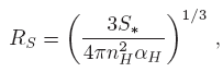
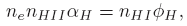
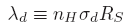
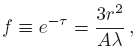
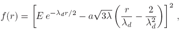
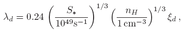
(11)This is a trascendental equation for (R0/RS) as a function of λd(see equation 9 ) that gives R0= RSfor λd= 0 (i.e., for no dust absorption), and can be inverted numerically for λd> 0. The result of this inversion is shown in Figure 1 .
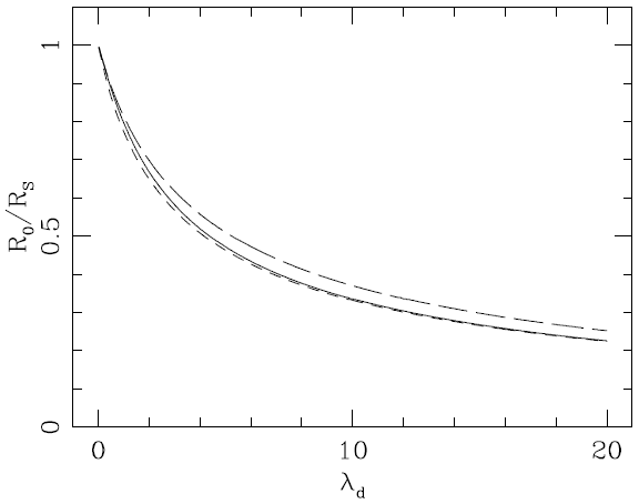
Fig. 1
Ratio between the outer radius of the ionized region R0and the (dust-free) Strömgren radius RS (see equation 1) as a function of the dust optical depth λd(see equation 9) obtained from the simplified (short dash line, see equation 11) and from the full version (solid line, see equation 16) of the Strömgren sphere analyis
The long-dash line corresponds to the outer radius obtained from the approximate solution of the radiative transfer problem obtained by Petrosian et al. (1972) , see equation (26).
Interestingly, in the Appendix of the paper by Franco et al. ( 1990 , which discusses the effect of dust on the radii of photoionized regions), equation (11) is derived through the simple argument that the dust will attenuate the ionizing photon rate S∗ by a factor of ≈ e−Td. This attenuated ionizing photon rate is then inserted in equation (1) to obtain the outer radius of the ionized nebula. The derivation above shows that the relation deduced by Franco et al. (1990) is indeed obtained from a proper “Strömgren sphere” analysis provided that the assumption of equation (10) is made. An explicit, approximate form for R0/RScan be obtained by taking the cube root of equation (11) and then expanding the exponential to second order in λdR0/RS. The resulting quadratic equation can then be inverted to obtain
 (12)
(12)This approximate equation follows well a numerical inversion of equation (11) for λd≤ 3, but has large deviations from the true solution for larger values of λd.
It is also possible to drop the assumption of equation (10) by noting that the number of absorptions due to photoionization out to a radius R is:
 (13)
(13)where THis the photoionization optical depth (see equation 4 ), from which we obtain
 (14)
(14)Using this value for TH (instead of setting TH = 0, as we have done for deriving equation 11 ), equation (8) then takes the form
 (15)
(15)Doing the integral, one obtains
 (16)
(16)where r0= R0/RS. This equation can be inverted numerically to obtain R0/RSas a function of λd. The results of this excersize are shown in Figure 1 , in which we see that for the displayed range of λd equation (16) gives very similar results to the ones obtained from equation (11) . The good agreement between equations (11) and (16) is an indirect justification of the approximation (see equation 10 ) used for deriving equation (11) .
In the following section we compare the outer radii R0 for the photoionized region obtained from equations (11) and/or (16) with numerical and analytic solutions of the radiative transfer+ photionization equilibrium problem.
3. THE RADIAL STRATIFICATION OF THE IONIZATION FRACTION
We now write the ionization balance condition ( equation 6 ) in terms of the (spatially dependent) H ionization fraction x = nHII/nH= ne/nH:
 (17)
(17)This quadratic equation for x can be inverted to obtain
 (18)
(18)with
 (19)
(19)We now use equations (19) and (6) to define
 (20)
(20)in terms of the dimensionless radius
 (21)
(21)and where the dimensionless parameter,
 (22)
(22)is the optical depth over a Strömgren radius RSassociated with photoionizations in the neutral gas. The above derivation is identical to the one of Raga (2015) and very similar to the one of Strömgren (1939) , who studied the case of a dust-free HII region. Now, from equation (4) we see that f obeys the differential equation
 (23)
(23)where x is given as a function of f and r by equations (18-20). This differential equation can be integrated numerically with the boundary condition f(0) = 1, but no exact analytic integral has been found.
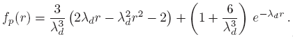
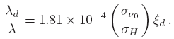
In order to obtain an approximate numerical integral, one expands the term in parentheses on the right hand side of equation (18) to first order in A, obtaining
 (24)
(24)This Taylor series expansion is compared with the exact form of 1 − x(A) (obtained from equation 18 ) in Figure 1 .
We now write A in terms of f and r using equation (20) and insert the result into equations (24) and (23) obtaining the differential equation
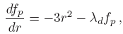 (25)
(25)where we have used the notation “f p ” in reference to the paper of Petrosian et al. (1972) . This equation can be directly integrated with the boundary condition f p (0) = 1 to obtain the approximate solution
 (26)
(26)This is the approximate analytic solution derived by Petrosian et al. (1972) . It can be easily shown that for λ d → 0 this solution converges to the f ( r ) = 1 − r 3, dust-free solution of Strömgren (1939) . Also, one sees that this solution gives an infinite optical depth (i.e., fp = 0, see equation 20 ) at a finite value rp , which can be obtained by inverting numerically the condition fp ( rp ) = 0 (see equation 26 ). The resulting values of rp as a function of λ d are shown in Figure 1 , in which we see that similar values to the r 0radii (resulting from global photoionization balance arguments, see equations 11 and 16 ) are obtained.
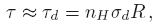
To obtain a better analytic approximation we follow Raga (2015) in approximating the x(A) dependence (see equation 18 ) with a three-segment interpolation of the form
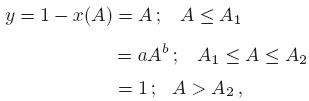 (27)
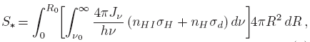
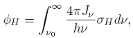
(27)with A 1= 0.1, A 2= 8.402, a = 0.316 and b = 0.5 (Raga 2015 used a b = 0.6 value, but as will be evident below, it is more convenient to choose a slightly different value for this coefficient).
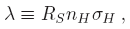
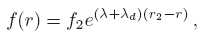
This approximation has a transition from the linear regime to a ∝ A 1/2power law at a neutral fraction y1 = A 1 = 0.1. The resulting interpolation is compared with the value of 1 − x ( A ) obtained using the exact form for x ( A ) (given by equation 18 ) in Figure 2 .
Fig. 2
The fraction 1 − x ( A ) of neutral H (where x = nHII / nH is the HII fraction) as a function of the A parameter (see equation 19 )
The exact solution ( equation 18 ) is shown with the solid curve. The linear approximation to 1 − x ( A ) ( equations 24 and 27 ) is shown with the thin, dotted line. The other two segments of the three-power law approximation ( equation 27 ) are shown with the thicker dotted lines.
With the approximate form for 1 − x ( A ) given by equation (27) , equation (23) can be integrated analytically to obtain
 (28)
(28)for r ≤ r 1(see equation 26 ),
 (29)
(29)for r 1< r ≤ r 2,
 (30)
(30)for r 2< r . In equation (29) the a constant has the value given after equation (27) , and we have considered the b = 1/2 case. It is also possible to obtain exact analytic integrals for b = n /2 values (with integer n ), but for other values of the power law exponent b (see equation 27 ) only approximate integrals can be obtained, resulting in more complex forms of the solution.
In equation (30) , f 2is the value given by equation (29) when evaluated in r = r 2. The matching consant E in equation (29) is given by
 (31)
(31)The switch between equations (28) and (29) occurs at a dimensionless radius r 1which is obtained from a numerical inversion of the equation
 (32)
(32)with fp ( r ) given by equation (26) .
The switch between equations (28) and (29) occurs at a dimensionless radius r 2which is obtained from a numerical inversion of the equation
 (33)
(33)with f ( r ) given by equation (29).
Approximate explicit forms for r 1and r 2can be obtained by expanding the corresponding equations (32 and 33) to first → fourth order around r 1,2= 1, and then finding analytically the roots of the resulting polynomials. We do not give here the results of this exercise, because they are hardly worthwhile.
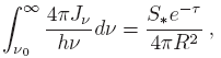
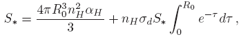
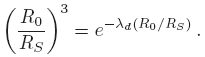
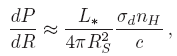
We can now calculate the radial dependence of the ionization fraction x (see equations 18 and 20) using the “exact” (i.e. numerical) solution of equation (23) and the two approximate analytic forms obtained for f ( r ) (the solution of Petrosian et al. 1972 given by equation 26 and the 3-segment approximation given by equations 28-30).
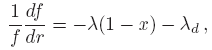
The three corresponding forms for x ( r ) obtained for the sets of parameters (λ = 100, λ d = 0.2), (λ = 1000, λ d = 0.2), (λ = 1000, λ d = 0.0) and (λ = 105, λ d = 20.0) are shown in Figure 3 . It is clear that the 3-segment approximation has a transition to neutral gas (i.e., for x → 0) that follows the exact solution in a more accurate way than the solution of Petrosian et al. ( 1972 , which reaches x = 0 at a finite radius).
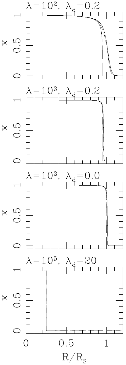
Fig. 3
The ionization fraction x = n HII /n H as a function of dimensionless radius r = R / RS (where RS is the Strömgren radius, see equation 1) obtained for the (λ, λ d ) parameter combinations given over each of the frames
In the four frames, the solid curve is the exact (i.e., numerical) solution, the long dash curve is the solution of Petrosian et al. (1972) and the short dash curve is the new, three-segment approximate analytic solution.
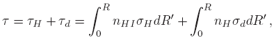
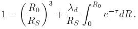
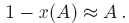
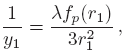
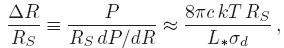
In Figure 4 , we show the radius R 0.9at which the ionization fraction has a x = 0.9 value as a function of λ d , for three values of the dimensionless parameter λ (=1000, 100 and 10) obtained from the exact (i. e., numerical) and from the 3-segment approximation (given by equations 28-30). These two solutions give almost indistinguishable results at the resolution of the figure. In the three plots we also show the R 0vs. λ d dependence obtained from the “dusty Strömgren sphere” analysis (see equation 16 and Figure 1 ). It is clear that for λ = 100 and 1000, the R 0.9radius closely follows the R 0vs. λ d dependence. For the lower, λ = 10 value, not surprisingly we find larger deviations between the R 0.9and R 0radii.
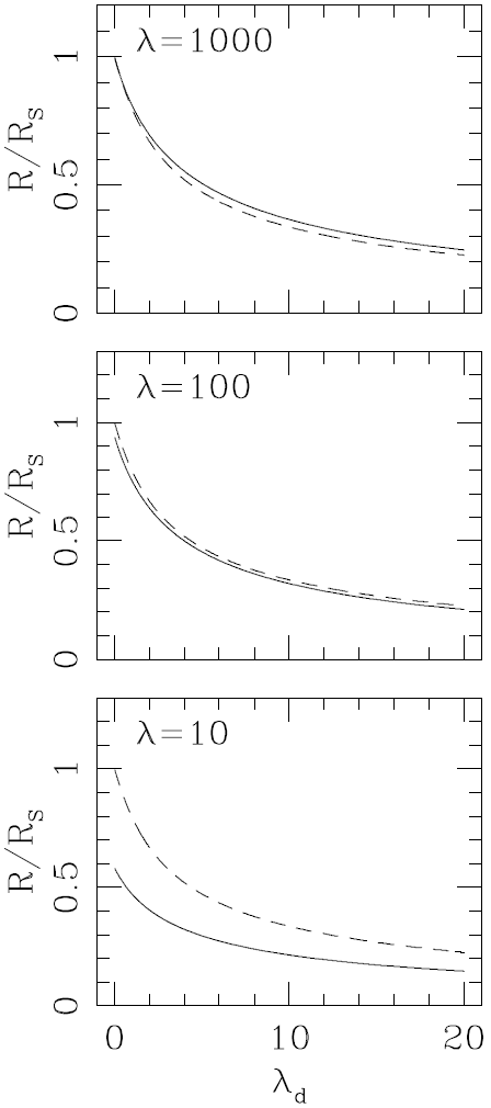
Fig. 4
The solid curves correspond to the radius R 0.9at which the ionization fraction reaches a x = 0.9 value as a function of λ d (see equation 9) for 3 different values of λ (see equation 22), λ = 1000 (top), 100 (center) and 10 (bottom)
The same curves (within the resolution of the graphs) are obtained from numerical integrations of the transfer equation (see equation 23) and from the threesegment, approximate analytic approximation (equations 28-30). The dashed lines show the outer radius R 0as a function of λd predicted from the “dusty Strömgren sphere” model ( equation 16 )
4. THE VALUES OF THE DIMENSIONLESS PARAMETERS
In § 3 we present solutions of the ionization structure of a homogeneous HII region which are given in terms of two dimensionless parameters:
-
λ = nHσHRS : the optical depth due to photoionization of H over a distance RS in a completely neutral medium,
-
λd = nHσdRS : the optical depth over a distance RS due to dust absorption.
Even though λ typically has values ≫ λ d , this does not necessarily imply that the dust absorptions are negligible, since within the nebula the neutral fraction of H is very low.
Also, in § 2, we presented a “dusty Strömgren sphere” model, in which the only dimensionless parameter that appears is λ d . This model is applicable for HII regions in the λ ≫ 1 limit.
The dimensionless parameter λ (see equation 22 ) has values
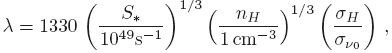 (34)
(34)where we have used typical parameters for a galactic HII region. The last term on the right (σ H /σʋ0) is the ratio between the average photoionization cross section (that has to be taken out of the integral in equation 2) and the Lyman limit cross section. This ratio is ≈ 1 for an HII region photoionized by a stellar source, but can have substantially smaller values for the case of a region photoionized by the “monster” (i.e., the accreting black hole) in the center of an active galaxy (which has a power law ionizing spectrum, see, e.g., Binette et al. 1993 ; Haro-Corzo et al. 2007 ). Therefore, for narrow line regions of AGNs we can have HII regions with substantially lower λ ∼ 10 → 100 values. Conversely, in very high density HII regions such as ultracompact regions within molecular clouds (see, e.g., Kurtz 2005 ), we can have very high densities, resulting in higher values, up to λ ∼ 105. Another way to have higher λ values is to have an HII region photoionized by a cluster with many O stars.
The average galactic dust absorption cross section per H atom at the Lyman limit has a value σ d ≈ 1.15 × 10⁻²¹cm2(see the discussion of Vasconcelos et al. 2011 ). Therefore, the dimensionless parameter λd (see equation 9 ) has a value
 (35)
(35)where ξd≤ 1 is the fraction of dust that survives within the HII region.
Combining equations ( 34 - 35 ) we obtain
 (36)
(36)In Figure 3 , we show the ionization stratifications of four different HII regions:
-
an HII region photoionized by a hard spectrum (resulting in λ = 100), and with average galactic dust abundance (so that λ d = 0.2, see equation 35 ),
-
an evolved galactic HII region (λ = 103) with average galactic dust abundance (λ d = 0.2),
-
an evolved galactic HII region (λ = 103) with no dust (λ d = 0),
-
an ultracompact HII region with density nH ≈ 106cm−3, with λ = 105and λ d = 20.
It is clear that in the last case the dust absorption has a very strong effect on the HII region, which has an outer radius of ≈ 1/4 of the Strömgren radius of a dust-free nebula.
5. APPLICABILITY OF A HOMOGENEOUS MODEL
The models described in this paper are limited to “Strömgren’s model”, i.e., to the case of a nebula with a homogeneous density and temperature. The way to obtain such a configuration is to “turn on” an O star within a homogeneous, neutral medium, and to wait for the “initial expansion” to take place. In this initial expansion, a fast R-type ionization front travels out and reaches the “initial Strömgren radius” (see, e.g., the lucid discussion in the book of Dyson & Williams 1980 ).
This initial Strömgren sphere does have a homogeneous density distribution, so that a homogeneous model is in principle applicable. However, at the ionization front it has a strong temperature gradient. The feedback of this temperature gradient on the ionization structure (through the rather weak temperature dependence of the H recombination coefficient) is not included in a homogeneous HII region model.
The other possibility is the application of a homogeneous model to the final, pressure equilibrium configuration (in which the HII region has expanded until it has reached pressure balance with the surrounding, neutral medium). In this final configuration, the almost constant temperature ( T ∼ 104K) resulting from the thermal balance guarantees an internal region with a quite homogeneous density. However, in the HII/HI transition region (in which the temperature has a transition from ∼ 104K to the ∼ 102→ 103K temperature of the neutral medium), the pressure balance condition implies a strong density gradient. This effect is of course not included in a homogeneous model.
Another effect that will introduce density gradients within the fully ionized region of a hydrostatic, dusty nebula is the radiation pressure on the dust grains. This effect was studied in detail by Draine (2011) . In order to evaluate the importance of the radiation pressure on dust grains let us consider the following, semi-qualitative analytic argument.
Let us assume that we have a low enough value of λd, so that the outer radius of the nebula has a value ∼ RS (i.e., the Strömgren radius of a dust-free nebula, see equation 1 ). This implies that the dust optical depth is at most of order 1, so that most of the stellar radiation (dominated by the non-ionizing photons) reaches regions close to the outer edge of the nebula. At radii close to RS , we then write the hydrostatic balance between the pressure gradient and the radiation pressure force as
 (37)
(37)where we have assumed a “grey” σ d ≈ 10−21cm2over all of the frequencies of the stellar spectrum. We can then calculate the radial scale ΔR of the pressure variations in the outer regions of the hydrostatic stratification as
 (38)
(38)where we have set P = 2 nHkT . Clearly, the pressure gradient induced by the radiation pressure force will be important for Δ R / RS ≈ 1 (or higher). Setting equation (38) equal to 1 and using equation (1) for RS , we then derive the density
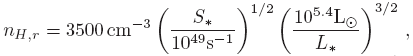 (39)
(39)above which the ionized region will develop an important pressure (and therefore density) gradient. In equation (39) we have used the values of S∗ and L∗ appropriate for an O5 dwarf, and a T = 104K temperature for the HII region.
If we insert the value of nH,r ( equation 39 ) in equation (35) , we obtain λ d ≈ 3.5. Therefore, for regions with values of λ d substantially above unity, we expect the constant density models (discussed in this paper) not to be applicable to the final, pressure equilibrium configuration of a nebula. However (as discussed above), even for lower λ d values, the homogeneous models do not describe appropriately the ionized to neutral transition in a pressure equilibrium nebula.
6. DISCUSSION
We have first presented a “Strömgren sphere” description for calculating the outer radius R 0of a homogeneous, dusty photoionized region (see § 2). In its most simple form (see equation 11 ), this approach leads to a simple, trascendental equation which can be inverted to obtain R 0/ RS (where RS is the Strömgren radius of a dust-free but otherwise identical region) as a function of the dust optical depth λ d = nHσdRS associated with Rs (see equation 35 ). We also find an approximate, explicit analytic inversion of this trascendental equation, which works well for λ d < 3 (see equation 12 ).
We have also studied a more detailed “Strömgren sphere” approach, which results in a different trascendental R 0/ RS vs. λ d relation (see equation 16 ). However, this relation gives similar results to the simpler equation (11) for the astrophysically relevant λ d range (see Figure 1 and § 3 ). Our simpler relation for the radius of a dusty Strömgren sphere was previously obtained by Franco et al. (1990) with a more qualitative approach.
We then compare the results of the “Strömgren sphere” approach with solutions of the associated radiative transfer problem (see equation 23 ), from which the ionization fraction x = nHII / nH is obtained as a function of radius. We integrate the resulting transfer equation numerically, and we also integrate it analytically using the approximation described by Raga (2015) , who studied the case of a dust-free HII region. This approximation is an improvement on the classical approximation of Strömgren (1939) , which was applied to the case of a dusty HII region by Petrosian et al. (1972) .
The presence of dust has a strong effect in the size of the ionized region for high nebular densities, as is the case in compact, ultra-compact and hypercompact HII regions (see the review of Kurtz 2005 ). Dust has of course been included in the past in detailed photoionization models of dense HII regions (see, e.g., Morisset et al. 2002 and Draine 2011 ).
The analysis presented above gives a clear physical picture of the transfer of ionizing photons in dusty HII regions, and results in relatively simple recipes ( equations 11 , 12 and 16 ) for obtaining the outer radius of such a region. We have also obtained a full analytic solution for the ionization fraction as a function of radius (see § 3), which can be useful for initializing numerical simulations of dusty, photoionized flows.
We end by noting again that homogeneous models (such as the ones described in the present paper) are a strong idealization of the situation found in real HII regions. Very special conditions are indeed necessary for such models to be directly applicable to observed objects (see the discussion of § 5).
We acknowledge support from the CONACyT grants 61547, 101356, 101975 and 167611 and the DGAPA-UNAMgrants IN105312 and IG100214. We acknowledge an anonymous referee for comments which lead to the discussion in § 5.
References
Binette, L., Wang, J., Villar-Martín, M., Martin, P. G., Magris, C. G. 1993, ApJ, 414, 535
Draine, B. T. 2011, ApJ, 732, 100
Dyson, J. E., Williams, D. A. 1980, “The Physics of the Interstellar Medium”, Manchester University Press, Manchester
Franco, J., Tenorio-Tagle, G., Bodenheimer, P. 1990, ApJ, 349, 126
Haro-Corzo, S. A. R., et al. 2007, ApJ, 662, 145
Hollenbach, D. J., Tielens, A. G. G. M. 1999, RvMP, 71, 173
Krumholz, M. R., McKee, C. F., Tumlinson, J. 2008, ApJ, 689, 865
Kurtz, S. 2005, in Massive star birth, a crossroads of astrophysics, eds. Cesaroni R. et al. (Cambridge: Cambridge Univ. Press), 111
Morisset, C. et al. 2002, A&A, 386, 558
Petrosian, V., Silk, J., Field, G. B. 1972, ApJ, 177, L69
Raga, A. C. 2015, RMxAA, in press
Sternberg, A., Le Petit, F., Roueff, E., Le Bourlot, J. 2014, ApJ, 790, 10
Strömgren, B. 1939, ApJ, 89, 526
Vasconcelos, M. J., Cerqueira, A. H., Raga, A. C. 2011, A&A, 527, 86