RECOMBINATION AND COLLISIONALLY EXCITED BALMER LINES
RECOMBINATION AND COLLISIONALLY EXCITED BALMER LINES
Revista Mexicana de Astronomía y Astrofísica, vol. 51, no. 2, 2015
Universidad Nacional Autónoma de México
Received: November, 24, 2014
Accepted: July, 28, 2015
Abstract: We present a model for the statistical equilibrium of the levels of H, considering recombinations to excited levels, collisional excitations up from the ground state and spontaneous radiative transitions. This problem has a simple "cascade matrix" solution, describing a cascade of downwards spontaneous transitions fed by both recombinations and collisional excitations. The resulting predicted Balmer line ratios show a transition between a low temperature and a high temperature regime (dominated by recombinations and by collisional excitations, respectively), both with only a weak line ratio vs. temperature dependence. This clear characteristic allows a direct observational identification of regions in which the Balmer lines are either recombination or collisionally excited transitions. We find that for a gas in coronal ionization equilibrium the Hα and Hβ lines are collisionally excited for all temperatures. In order to have recombination Hα and Hβ it is necessary to have higher ionization fractions of H than the ones obtained from coronal equilibrium (e.g., such as the ones found in a photoionized gas).
Keywords: Herbig-Haro objects, hydrodynamics, ISM: individual objects (HH1, HH2), ISM: kinematics and dynamics, shock waves.
Resumen: Presentamos un modelo para el equilibrio estadístico de los niveles de H, considerando recombinaciones a los niveles excitados, excitaciones colisionales partiendo desde el nivel fundamental y transiciones radiativas espontáneas. Este problema tiene una simple solución en términos de la "matriz de cascada", que describe una cascada de transiciones espontáneas alimentada tanto por recombinaciones como por excitaciones colisionales. Las predicciones resultantes de cocientes de líneas de Balmer muestran una transición entre un régimen de baja temperatura y uno de alta temperatura (dominados por recombinaciones y por excitaciones colisionales, respectivamente), ambos con sólo una dependencia débil de la temperatura. Esta clara característica permite una diferenciación observacional directa entre regiones de líneas de Balmer de recombinación y regiones con líneas excitadas colisionalmente. Encontramos que para un gas en equilibrio coronal las líneas de Hα y Hβ se excitan colisionalmente a todas las temperaturas. Para obtener líneas de Hα y Hβ de recombinación, es necesario tener fracciones de ionización de H subtancialmente mayores que la de equilibrio coronal (por ejemplo, como las presentes en un gas fotoionizado). Received 2014 November 24. Accepted 2015 July 28. 1. INTRODUCTION
1. INTRODUCTION
Seaton (1959a,b) presented calculations of the recombination cascade of hydrogen (H), considering the transitions between different principal (i.e., energy) quantum numbers n , and assuming an equilibrium distribution between the angular momentum levels l corresponding to a given n . The effect of considering explicitly the different values of l was studied by Pengelly & Seaton (1964). Brocklehurst (1970, 1971) calculated the statistical equilibrium for the ( n, l ) levels of H, also including redistribution between the different l values (at constant n ) due to collisions with protons, as well as collisions with electrons producing transitions between different n values. More recent results on the recombination cascade of hydrogenic ions (including redistribution between different angular momentum levels through collisions with protons) are presented by Storey & Hummer (1995). Even more recently, Storey & Sochi (2014) analyzed the collisional excitation and recom- bination of the excited levels of H resulting from non- thermal electron distribution functions.
Aggarwal (1983) calculated the electron impact collisional excitation rates for the 1 → 2 and 1 → 3 transitions, and suggested that they could have an important effect on the prediction of low lying lines of H. This effect was evalued in more detail by Hummer & Storey (1987). More recently, Stasin´ska & Izotov (2001) and Luridiana et al. (2003) calculated photoionized region models from which they concluded that for some parameters the collisional excitations from the n = 1 levels can have an effect of ≈ 5% in the predicted Balmer line intensities.
The effect of collisional excitations upwards from the n = 1 levels of H of course can have a dominant effect in astrophysical shocks. Immediately after the shock, one has a high temperature region (of ≈ 105 K for a 100 km s−1 shock) in which H can be partially neutral, though rapidly becoming collisionally ionized. In this region, the 1 → n electron collision excitations dominate over the recombinations to the excited levels of H. This effect was included in the shock models of Raymond (1979), who added the contribution of the collisional excitations of the low lying levels of H to the recombination cascade.
In this paper, we present a simple model for the statistical equilibrium of the excited levels of H including both the recombinations and the upwards electron collisional excitations from the ground state. This model can be solved with the traditional “cascade matrix” solution (see, e.g., the book of Osterbrock & Ferland 2006), with a cascade of downwards spontaneous transitions which is fed both by recombinations and by collisional excitations from the ground state.
In § 2, we discuss the statistical equilibrium and the calculation of line emission coefficients, giving the results obtained for the Hα emission. In § 3, we present the results obtained for the Hα/Hβ and Hβ/Hγ ratios. These results are summarized in § 4. Finally, the paper has two appendices which give all the necessary parameters for solving the 5-level H atom problem, and analytic fits giving the predicted line intensities and/or line ratios as a function of temperature and ionization fraction of the gas.
2. THE STATISTICAL EQUILIBRIUM AND THE EMISSION COEFFICIENTS
Let us consider the statistical equilibrium for the excited levels of H, under the assumption that they are populated by recombinations (due to electron collisions with HII), spontaneous transitions from higher energy levels and upward collisional excitations from the ground ( n = 1) state, and depop- ulated only by downwards spontaneous transitions. For the energy level k > 1, we then have:
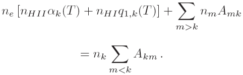 (1)
(1)In this equation, αk ( T ) is the radiative recombina- tion coefficient to level k , q1, k ( T ) is the electron collisional excitation coefficient for the 1 → k transition, the Akm are the Einstein spontaneous transition coefficients, ne is the electron number density, nHII is the ionized H number density, and nHI the neutral H density.
In this equilibrium equation, we neglect the col- lisional transitions between the excited levels, and the photo and collisional ionizations from the excited levels. Furthermore, we assume that the number density of the n = 1 level is equal to nHI (i.e., that the vast majority of neutral atoms are in the ground state). This amounts to a “low density regime” assumption, in which the only active collisional transitions (as well as the photoionizations) are the ones starting from the ground state. This is a clearly valid assumption for the permitted transitions of H at interstellar medium densities.
The solution to the statistical equilibrium equa- tions (see equation 1) can be written as:
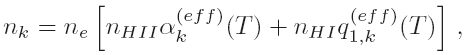 (2)
(2)with an effective recombination coefficient defined in the usual way as:
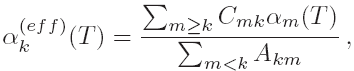 (3)
(3)and an analogously defined effective collisional excitation coefficient:
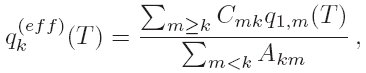 (4)
(4)in terms of the “cascade matrix” Cmk . This matrix can be calculated recursively by first computing the probability Pkm of having a direct k → m transition:
 (5)
(5)and then using these branching ratios to calculate iteratively the terms of the cascade matrix
 (6)
(6)which give the probability of having a k → m transition either directly or by a cascade of intermediate spontaneous transitions. The diagonal elements of the matrix are given a value of 1 (i.e., Ckk = 1). A discussion of the cascade matrix formalism can be found in the book of Osterbrock & Ferland (2006).
Once the effective recombination and collisional excitation coefficients have been obtained, one can calculate the emission coefficients for the k → m transition as:
 (7)
(7)where
and
(with Ekm being the energy of the k → m transition).
We should note that in the above derivation we have considered the energy levels of H to have equilibrium populations for their angular momentum levels (i.e., that for a given n, the angular momentum levels l have relative populations proportional to their statistical weights 4l + 2). As shown in the classical paper of Brocklehurst (1971), more detailed models for the population of the levels of H (considering the transitions between the different angular momenta due to collisions with protons) give small deviations (of order ∼ 2%) in the predictions of the ratios between the lower lying Balmer line intensities. We do not consider these effects in the present paper.
With the Einstein coefficients Akm , the collisional excitation coefficients q 1, m ( T ) and the recombination coefficients α m ( T ) we can calculate the effective recombination and collisional excitation coefficients α m ( eff ) ( T ) and qm ( eff ) ( T ) (given by equations 3 and 4, and the recombination and collisional enegy rates ( Er km and Ec km , see equation 7). As described in detail in Appendix A, we have done this calculation for the n = 1 → 5 levels of H, considering “case A” (i.e., with optically thin lines) and “case B” (in which the Lyman transitions are optically thick).
In Figure 1, we show the recombination and collisional energy rates Er H α and Ec H α (see equation 7) as a function of temperature for “case B” (left, optically thick Lyman lines) and “case A” (right, optically thin Lyman lines). For the “case B” coefficients, we have also calculated analytic fits, which are described in Appendix B (dashed lines in the left panel of Figure 1). It is clear that for temperatures below ≈ 104K the recombination energy rate is dominant, but for larger temperatures the collisional excitation energy rate dominates by many orders of magnitude. Because of this, even if the product nenHI is very small (i.e., because H is mostly ionized), the collisional excitation contribution to the Hα emission becomes dominant at high enough temperatures. This effect is discussed in more detail in the following Section.
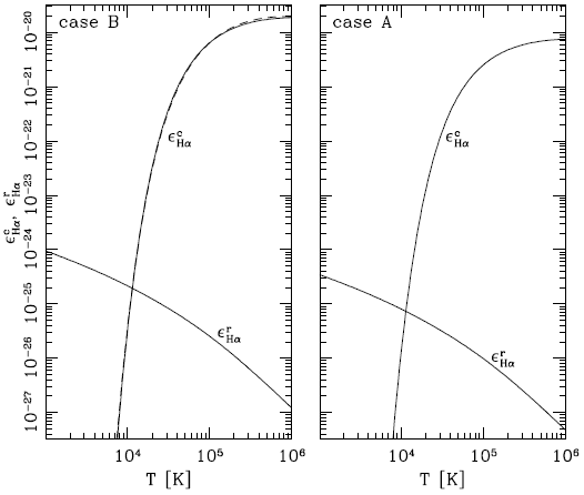
Fig. 1
Contributions to the Hα emission coefficients of the recombination cascade ( Er H α) and the collisional excitation cascade ( Ec H α) as a function of temperature, for the “case B” (left) and “case A” (right) approximations (see the discussion in § 2).
The solid lines give the numerical results from the cascade calculations, and the dashed lines give the analytic fits to the “case B” results, described in Appendix B (left frame).
3. THE Hα/Hβ AND Hβ/Hγ LINE RATIOS
We now assume that most of the free electrons come from the HII, and set ne = nHII = xnH and nHI = (1 − x ) nH , where nH is the total H density. Then, from equation (7) we obtain the line emission coefficients as:
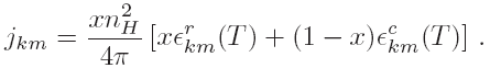 (8)
(8)Therefore, the observed ratios of optically thin lines from a homogeneous region (which are proportional to the ratios of the corresponding emission coefficients) are only a function of the temperature T and the H ionization fraction x (since the dependence on the H density nH cancels out as all emission coefficients are proportional to n 2 H , see equation 8).
In Figures 2 and 3 we show the resulting Hα/Hβ and Hβ/Hγ ratios as function of T and x for the “case B” (Figure 2) and “case A” (Figure 3) approximations (see § 2 and Appendix A). It is clear that at temperatures smaller than ≈ 104K, we obtain an almost constant value for the line ratios (as has been shown repeated times for the H recombination lines, see e.g. Brocklehurst 1971), a region around T ≈ 104K in which the line ratios show a relatively strong dependence on both x and T , and a high temperature regime in which the line ratios again are almost constant.
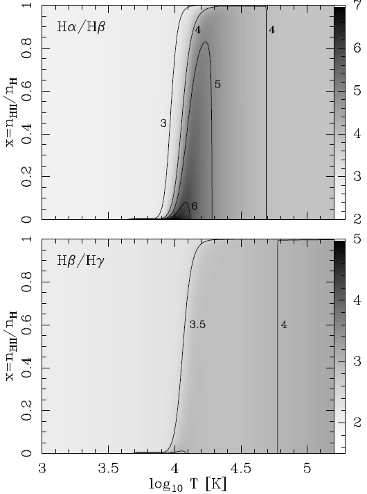
Fig. 2
Case B (i.e. optically thick Lyman lines) Hα/Hβ (top) and Hβ/Hγ ratios (bottom) as a function of temperatura and H ionization fraction ( x = nHII / nH ) calculated with the emission coefficients given by equation 8.
The line ratios are shown with labeled contours and with linear greyscales given by the bars on the right.
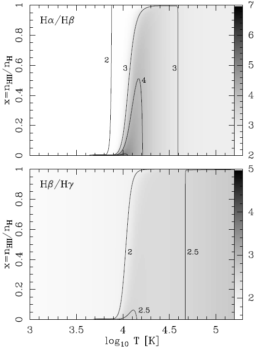
Fig. 3
Case A (i.e. optically thin Lyman lines) Hα/Hβ (top) and Hβ/Hγ ratios (bottom) as a function of temperatura and H ionization fraction ( x = nHII / nH ) calculated with the emission coefficients given by equation 8
The line ratios are shown with labeled contours and with linear greyscales given by the bars on the right.
This behavior is also shown in Figures 4 (case B) and 5 (case A), in which the line ratios are shown as a function of temperature for three fixed values of the ionization fraction of H ( x = 10−3, 0.5 and 0.999). It is clear that the line ratios have a “low temperature regime” (dominated by the recombination cascade) and a “high temperature regime” (dominated by the collisional excitation cascade) in which the line ratios are independent of the H ionization fraction x . In the transition between these two regimes, the line ratios depend on both T and x .
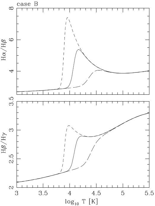
Fig. 4
Case B Hα/Hβ (top) and Hβ/Hγ ratios (bottom) as a function of temperature for three different values of the H ionization fraction: x = nHII / nH = 0.999 (long dashes), 0.5 (solid line), and 0.001 (short dashes).
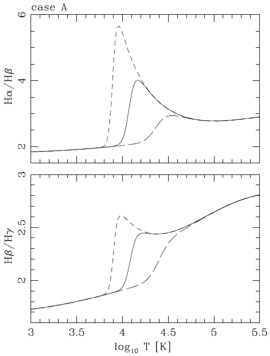
Fig. 5
Case A Hα/Hβ (top) and Hβ/Hγ ratios (bottom) as a function of temperature for three different values of the H ionization fraction: x = nHII / nH = 0.999 (long dashes), 0.5 (solid line), and 0.001 (short dashes).
In the low temperature regime, the temperature dependence of the line ratios is weak, reflecting the weak (and similar) temperature dependencies of the recombination coefficients to the excited levels of H. In the high temperature regime, the temperature dependence of the line ratios is also small. This is because the populations of the excited levels m through collisional excitations are dominated by the direct excitation to level m . Therefore, the temperature dependence of the nm / nk ratio (which determines the ratios of lines starting from the pair of levels) is given by a term of the form:
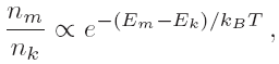 (9)
(9)where we have neglected the (weak) temperature dependence of the collisional excitation coefficients (see Appendix A). It is clear that for T ≫ ( Em − Ek )/ kB (where kB is Boltzmann’s constant) the line ratios basically become independent of T . These temperatures are ( E 4 − E 3)/ kB = 7681 K for the Hα/Hβ ratio and ( E 5 − E 4)/ kB = 3551 K for the Hβ/Hγ ratio. In Appendix B we give approximate analytic forms for calculating the case B Hα/Hβ and Hβ/Hγ ratios.
From Figures 2, 3, 4, 5 we see that for ionization frac- tions x → 1, the line ratios preserve their recombination cascade values up to increasing values of the temperature. This result is intuitively clear, since for x = 1 (i.e., for a neutral fraction 1 − x = 0) no collisional excitations (up from the n = 1 level) take place. This is seen in equation (8), from which for x = 1 we obtain jkm ∝ Er km ( T ).
In order to quantify this effect, we calculate the neutral fraction 1− xc (as a function of T ) for which the Hα emission has equal contributions from collisional excitations and from the recombination cascade. We find this neutral fraction by setting the two terms within the square brackets of equation 8 equal to each other, from which we obtain:
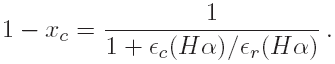 (10)
(10)From our 5-level H atom calculation, we compute the 1− xc neutral fraction (at which the recombination cascade and collisional excitation contributions to Hα are equal) as a function of temperature, and show the results in Figure 6.
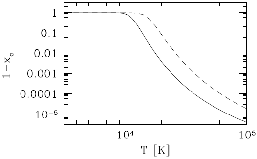
Fig. 6
The solid line shows the neutral H fraction 1− xc (above which the contribution of collisional excitation to the Hα emission dominates over the recombination cascade) as a function of T .
Indistinguishable 1 − xc vs. T curves are obtained from cases A and B. The dashed line shows the neutral H fraction given by the coronal ionization equilibrium condition. The coronal equilibrium neutral fraction is higher than 1− xc at all temperatures.
This figure can be interpreted as follows. For neutral fractions larger than 1 − xc , the Hα emission is dominated by the collisional excitation contribution. Therefore, for temperatures T < 104 K, in order to have an important contribution from collisional excitations one needs to have neutral fractions very close to 1 (so that the recombination cascade term of equation 8 becomes very low). However, for T > 104 K the collisional excitation contribution becomes dom- inant for monotonically decreasing 1− xc values (see Figure 6).
Interestingly, if we compare the temperature de- pendence of the neutral fraction corresponding to coronal ionization equilibrium (i.e., the ionization state determined from the equilibrium between collisional ionizations and radiative recombinations of H), we see that coronal equilibrium gives higher neutral fractions at all temperatures. Therefore, the Hα emission of a gas in coronal ionization equilibrium is dominated by the collisional excitation contribution at all temperatures.
4. DISCUSSION
We have derived a simple model of a spontaneous transition cascade fed by both recombinations and electron impact excitations upwards from the ground level of H.With this model, the level populations and the line emission coefficients can be written in terms of the usual “effective recombination coefficients” (equation 3) and of equivalently defined “effective collisional excitation coefficients” (equation 4).
We calculated the recombination and the collisional contributions to the emission coefficients of the Hα, Hβ and Hγ lines as a function of temperature and H ionization fraction x = nHII / nH and found that the Balmer line ratios have a transition from a “low temperature” to a “high temperature” regime, with approximately temperatura-independent ratios in both regimes. The low temperature regime of course corresponds to the recombination cascade, which is known to produce line ratios with only a weak temperature dependence. The high temperature regime corresponds to collisionally excited H lines in the regime in which kT is much larger than the energy difference between the upper levels giving rise to the pair of lines in the ratio (for which the line ratio again shows only a weak dependence on temperature).
The details of the transition between the low and the high temperature regimes of the line ratios depend on the ionization fraction x of the gas (see Figures 2 and 3). For low values of x, the Hα/Hβ and Hβ/Hγ line ratios show strong peaks as a function of temperature, before settling onto the high temperature regime values. These peaks disappear for values x ≈ 1, and a monotonic transition between the low and high temperature line ratio regimes is then obtained (see Figures 4 and 5).
The existence of this clear transition between a low and a high temperature regime (in which the H level populations are dominated by recombinations and by collisional excitations, respectively) has interesting implications for observations of shock waves. For example, in high angular resolution observations of Herbig-Haro (HH) objects one might detect both the Balmer line emission of the hot, immediate post-shock region (with temperatures in excess of ≈ 105K, where one would see the effect of the collisional excitations) and of the cooler (≈ 103 → 104K) recombination region (dominated by the recombination cascade). The first region would be characterized by an Hα/Hβ ratio of ≈ 4 (see the high temperature regime of this ratio in Figure 4), and the second region by the recombination Hα/Hβ ≈ 2.8 value (see the low temperature regime in Figure 4 or, e.g., Pengelly & Seaton 1964). This effect is seen in the new Hα and Hβ images of HH 1 and 2 of Raga et al. (2015).
Our results might also be applicable for observations of Balmer dominated, non-radiative shocks (in which the Balmer line emission is due to collisional excitation in the immediate post-shock region, see, e.g., the reviews of Raymond 2001 and Heng 2010). With high signal-to-noise observations of the Hα, Hβ and Hγ lines, it would be possible to use the predictions of the high temperature regime Hα/Hβ and Hβ/Hγ line ratios (see the T > 105K region of Figure 4 and the interpolations given by equations B18-B19) to obtain a simultaneous determination of the extinction and of the average temperature of the emitting gas.
Very interestingly, we find that for a gas in coronal ionization equilibrium (i.e., the equilibrium re- sulting from the balance between collisional ionizations and radiative recombinations of H) the Hα emission is dominated by the collisional excitation contribution (see Figure 6). In order for the recombination cascade to have a dominant contribution to the Hα emission one needs a gas with considerably higher ionization fraction (i.e., lower neutral fraction) than the coronal equilibrium value. This situation is found, e.g., in photoionized regions (in which high ionizations are found even for relatively low temperature values as a result of the high photoionization rate) and in recombination regions of shock waves (in which the recombining gas relaxes toward, but never reaches, coronal equilibrium). On the other hand, the immediate post-shock collisional ionization regions have neutral fractions higher than coronal equilibrium, so that they have an Hα emission which is clearly dominated by the collisional excitation contribution.
Finally, the work presented in this paper gives a straightforward method for calculating the Balmer line emission from shock wave models. This can be done by solving the recombination+collisional excitation cascade model (for which all parameters are given in Appendix A) or by using the analytic fits which have been obtained for the case B emission coefficients and line ratios (see Appendix B).
Acknowledgement
We acknowledge support from CONACyT grants 101356, 101975 and 167611, DGAPA-UNAM grants IN105312 and IG100214. We an acknowledge anonymous referee for comments which led to the results presented in Figure 6.
References
Aggarwal, K. M. 1983, MNRAS, 202, 15
Brocklehurst, M. 1970, MNRAS, 148, 417
Brocklehurst, M. 1971, MNRAS, 153, 471
Dere, K. P., Landi, E., Mason, H. E., Monsignori Fossi, B. C., & Young, P. R. 1997, A & AS, 125, 149
Heng, K. 2010, PASA, 27, 23
Hummer, D. G., & Storey, P. J. 1987, MNRAS, 224, 801
Landi, E., Del Zanna, G., Young, P. R., Dere, K. P., Mason, H. E., & Landini, M., 2006, ApJS, 162, 261
Luridiana, V., Peimbert, A., Peimbert, M. & Cervino, M. 2003, ApJ, 592, 846
Osterbrock, D. E., & Ferland, G. J. 2006, Astrophysics of gaseous nebulae and active galactic nuclei, University Science Books (Sausalito, USA)
Pengelly, R. M., & Seaton, M. J. 1964, MNRAS, 127, 165
Raga, A. C., Reipurth, B., Castellanos-Ramírez, A., Chiang, H-F, & Bally, J. 2015, ApJ, in press
Raymond, J. C. 1979, ApJS, 39, 1
Raymond, J. C. 2001, SSRv, 99, 209
Seaton, M. J. 1959a, MNRAS, 119, 81
Seaton, M. J. 1959b, MNRAS, 119, 90
Stasinska, G., Izotov, Y. 2001, A & A, 378, 817
Storey, P. J., Sochi, T. 2014, MNRAS, in press
APPENDICES
A. COEFFICIENTS FOR THE RECOMBINATION AND COLLISIONAL EXCITATION CASCADE
In this Appendix we give the atomic parameters and coefficients used to calculate the statistical equilibrium for the n = 3 → 5 levels of H (see equations 2-6). We have taken the Einstein A coefficients and the collision strengths Ω by appropriately grouping the parameters given in the Chianti database (Dere et al. 1997; Landi et al. 2006). To describe the temperature dependencies of the collision strengths of the 1 → k transitions we calculated least squares polynomials of the form
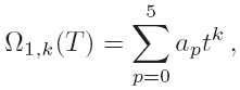 (A11)
(A11)with t = log10( T /104K) in the T = 103 → 108K temperature range. The values of the ak coefficients for the transitions to levels k = 2 → 5 (as well as the A coefficients) are given in Table 1.
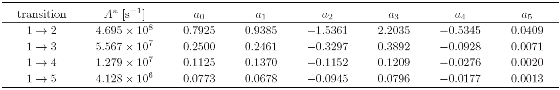
aAlso: A 32 = 4.410×10⁷s−1, A 42 = 8.419×10⁶s−1, A 43 = 8.986×10⁶s−1, A 52 = 2.530×10⁶s−1, A 53 = 2.201×10⁶s−1 and A 54 = 2.699 × 10⁶s−1.
The q 1, k collisional excitation coefficients were then calculated with the standard relation
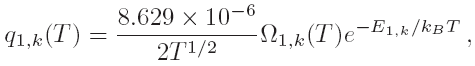 (A12)
(A12)with T in K, and where we considered that the statistical weight of the ground state is g 1 = 2.
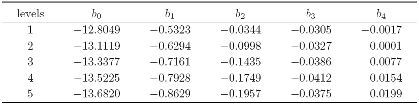
We calculated the recombination coefficients α k to the excited levels of H following Seaton (1959a), and we then calculated least squares fits of the form
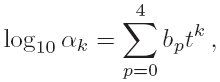 (A13)
(A13)with t = log10( T /104K), in the T = 103 → 106K temperature range. The coefficients for the polinomials interpolating the α k ( T ) are given in Table 2 for k = 1 → 5.
With these coefficients we calculated the recombination cascade and the collisionally excited cascades described in § 2. The “case A” calculation was done with the Einstein A coefficients given in Table 1, and the “case B” calculation was done setting to zero the A coefficients of the Lyman transitions (i.e., setting Ak ,1 = 0 for all k ).
B. ANALYTIC FITS FOR THE “CASE B” EMISSION
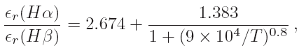
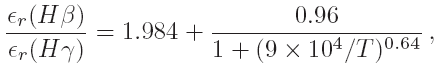
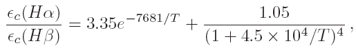
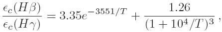
In this Appendix we present analytic fits to the temperature dependence of the “case B” recombination and collisional excitation contributions to the Hα emission and to the temperature dependence of the Hα/Hβ and Hβ/Hγ ratios of the “case B” recombination and collisional contributions:
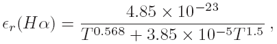 (B14)
(B14)to better than 3% in the 103 → 106K temperature range,
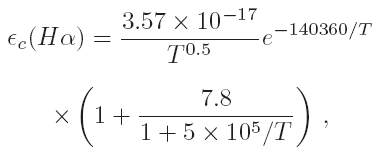 (B15)
(B15)to better than 8% in the 104 → 106K temperature range,
 (B16)
(B16)to better than 1% in the 103 → 106K temperature range,
 (B17)
(B17)to better than 0.7% in the 103 → 106K temperature range,
 (B18)
(B18)to better than 0.7% in the 104 → 106K temperature range, and
 (B19)
(B19)to better than 0.8% in the 104 → 106K temperature range.
In these interpolation fomulae, T is the temperature in K. The fits to the recombination and collisionally excited Hα emission (equations B14-B15) are shown in Figure 1.