INTRODUCTION

One of the most important political debates in modern Mexico is focused on income inequality. The high levels of poverty and the increasing accumulation of wealth in a small percentage of the population, combined with the failed war on drugs and widespread corruption, have created the conditions for social discontent and rampant crime in some areas of the country. Historically, since the Mexican Revolution, the government has pursued an assertive policy agenda to mitigate poverty through comprehensive social programs such as Opportunities and Prospera. However, reducing inequality is a difficult and more complex issue to address.

In 2012, when Enrique Peña Nieto became President of Mexico, he promoted right away an aggressive reformist agenda, affecting several protected sectors of the economy in an attempt to modernize Mexico’s economic system. The reforms that he negotiated and implemented were in areas such as Energy, Education, and a comprehensive Tax Reform. It was at the beginning of 2014 when most of these reforms were in effect. These changes were necessary for the country to be competitive and to modernize some of its most important economic sectors. Nevertheless, these reforms were received with skepticism for a variety of reasons. The Energy Reform affected an industry considered as one of the most important sources of wealth of the nation, and that has been administered by a company fully controlled by the government for more than 75 years until this reform took place.

In the case of the Education Reform, which aim is to modernize and standardize public education by implementing evaluations for professors across the country and by defining methods of promotion and dismissal linked to student performance, was opposed by the National Union of Education Workers, the largest labor union in Latin America and the most powerful in Mexico, which strong opposition delayed its implementation.

Regarding the Tax Reform, this was perhaps the reform that was more anticipated as the taxation system in Mexico was unnecessarily complicated and was in need of constant amendments to maintain relevance. The argument was that even with these recurrent changes, the Mexican taxation system ability to raise acceptable taxes was far worse that similar developing economies.

With all these structural changes taking place simultaneously in a developing economy, it is critical to ask about the effects of these changes to the welfare of society. The focus of this paper is to measure the effect of the reforms on social inequality, in particular the Tax Reform, while controlling for income levels.

The importance of the relationship of income and inequality has been defined in the literature extensively, starting with Kuznets (1955) who suggested for the first time a relationship between these two economic measurements. Kuznets explained that as income increases, inequality increases to a certain level, and then begins to decrease, creating an inverted U-shaped pattern. This conclusion was based on the transition of economies from the pre-industrial to the industrial system, with a period of stabilization when the benefits of industrialization spread across society.

Conceição & Galbraith (2001) expanded this theory with an Augmented Kuznets curve. They found evidence indicating that after the inverted U-shaped pattern was observed, economies have periods of increasing inequality and income, a sign of more advanced economies, moving to technological intense industries and capital goods.

So the question remains about how the new policy implementation affected the levels of inequality in Mexico and how income and inequality performed during this period of study.

Three years after these fundamental reforms were implemented, we analyze if there are significant changes to the levels of inequality in Mexico, as a whole and on distinctive groups.

To summarize, the main questions explored in this paper are the following:

• • Is there evidence that income inequality has increased in general, in the rural and urban sectors and by occupation in Mexico, for the period of 1996 to 2016?

  • Is there evidence that the income-inequality relationship in Mexico is presenting an Augmented Kuznets Curve for the period 1996 to 2016?

  • Is there evidence that income inequality in Mexico has increased significantly after the reforms of 2014, based on a sub-national level analysis of inequality?

MEASURING INEQUALITY

Following Foster’s taxonomy (2006), there are six commonly used measures of income inequality. These are fractiles¹, coefficient of variation, Lorentz curve, Theil index, social welfare function, and Gini coefficient. The last one is the most recognized measure of inequality and the one that will be applied in this paper. The method to calculate the Gini coefficient incorporates all the observations and their differences in magnitude. This is accomplished by making pairwise comparisons among pairs of income values, in an exhaustive process. Then, the absolute differences of these comparisons are added together and the total is divided by the square of the total number of elements in the sample, multiplied by the mean of the income. This is to normalize the coefficient to range from 0 to 1.

The formula to estimate the Gini coefficient based on Sen (1973) is:

Theoretically, a Gini coefficient with value 0 means no inequality; everybody is receiving the same income. The higher the value of the Gini coefficient, the higher the inequality. The lower the value of the Gini coefficient, the lower the inequality among the members of the group of interest.

INEQUALITY AND INCOME AS A RELATIONSHIP OF INTEREST

When studying income inequality, it is inevitable to recognize the strong relationship that it has with the income of the group of interest. Kuznets (1955) studied for the first time the relationship between income and inequality, and its link to the level of industrialization and development of the economy.

The hypothesis was that as economies evolved from an agricultural based (or pre-industrial) economy to an industry based economy, with increases in income as a consequence, inequality will initially increase, and then will decrease once the transition process has settled. “The underlying assumption is that income differentials between the agricultural and industrial sectors are such that they encourage migration of human capital from one sector to the other, triggering a period of generalized high inequality. But once the simultaneous processes of migration and urbanization settle down, economic wellbeing continues to grow while inequality is reduced” (Brussolo, 2011:15).

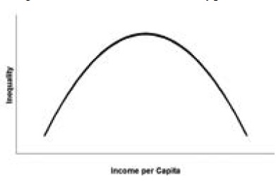
Figure 1:
Kuznets Inverted U Hypothesis

illustrates this notion, known as the Kuznets Inverted U Hypothesis.

Recent studies have found empirical evidence that suggests that after the transition of the traditional economic sector to a more modern sector when inequality increases and then decreases, there is a change in the Kuznets curve. More modern economies, which have transition to the industrial sector long time ago, will experience an Augmented Kuznets curve (Conceição & Galbraith, 2001), when the inequality will increase once again, as those economies changed to be suppliers of capital goods and technology.

DATA AVAILABILITY

This analysis is based on a very rich database, which has been rarely used for this type of research containing representation of the 32 Mexican States and a set of self-represented cities. This database includes detailed information of individual salaries and earnings from 1996 to 2016, from a series of surveys planned and executed by the INEGI (National Institute of Statistics, Geography and Informatics) in collaboration with the Mexican Labor Department. These surveys are the National Employment and Occupation Surveys, performed every quarter using rotated panels in which the households that are part of the sample are maintained for five quarters, in a way that in the following year, 20% of the sample will consist of the same elements. The sample process involves stratified, multistage clusters with statistical representation per state in urban and rural areas, with an average of more than 150,000 individuals surveyed per quarter².

This survey contains information about gender, age, occupation, educational attainment, as well as salaries and remunerations for individuals 15 years and older³. For this research, we utilized the second quarter of each year to avoid seasonal effects in the income⁴.

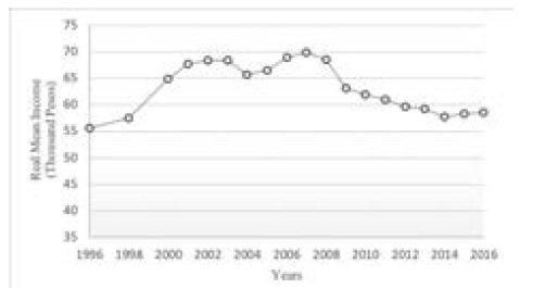
Figure 2:
Mean real income 1996-2016

Figure 2 shows the real income per year in Mexican pesos⁵. The trend indicates an increase of real income in the middle of the period, and a drop in 2009, corresponding with the effects of the last global recession. The salaries have not recuperated yet to their previous level, and they have been steady since 2012.

ADDRESSING THE RESEARCH QUESTIONS

The first step to evaluate inequality levels, is to estimate Gini coefficients for the country as a whole for the period of study, then calculate them by sector (Rural or Urban), by occupation (Employees, Business Owners and Independent Workers) to identify patterns and affected groups. Gini coefficients for each of the 32 states per year were generated to be analyzed and used for a regression discontinuity model. The estimation of Gini Coefficients allowed us to take full advantage of the richness of the survey data.

There are two different approaches to calculate income inequality using this data, one is based on individual surveys, using individual income, obtaining a measure of inequality among income earners. Those reporting zero income are not included in this inequality estimate. The second approach calculates inequality among households. For this estimation, first it is necessary to group individual surveys per household, then add the income for the household (from income earners), and divide the total income among the household members, calculating an average income per member of the household.

This calculation reduces the dispersion of the variable as the income from earners will be distributed equally among all household members including dependents and members not working. This second approach has an effect on how the income inequality is calculated and how much dispersion is reflected, but the underlying principle provides more realistic estimates of the income per family.

INCOME INEQUALITY IN MEXICO FOR THE PERIOD 1996 TO 2016

Inequality in Mexico per household was estimated and it is presented in Figure 3. During the period of study, inequality decreased significantly at the beginning, stagnated for few years and then it increased for the last segment of the period. The highest level of inequality was reported in the first year of the series with 0.51 (1996); the lowest was reported in 2009 with a Gini coefficient of 0.38.

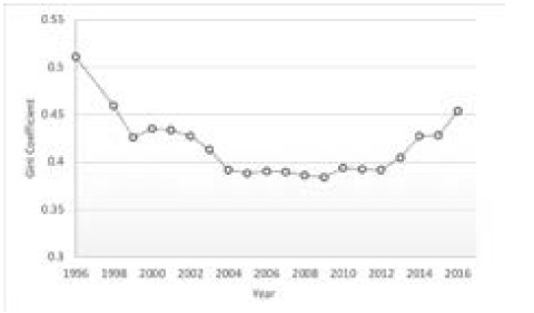
Figure 3:
Gini coefficient per household 1996-2016

The inequality levels in the rural and urban sectors of Mexico show a similar pattern for the period of study but with higher inequality levels for the urban sector than the rural sector⁶. Figure 4 reports the levels of inequality on both sectors. The gap between rural and urban inequality is the highest in 1998 with more than 0.10 differential in the coefficient. The lowest gap is in 2016, with 0.01 difference in inequality, with a notorious decrease in the difference in inequality between sectors in recent years. It is interesting to see that it was not the urban inequality the one that was reduced, but it was the rural inequality the one that increased almost to match the level of inequality in the urban sector.

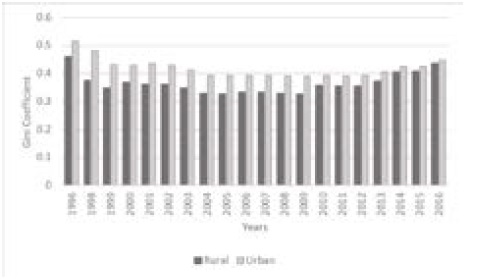
Figure 4:
Rural and urban inequality in Mexico 1996-2016

For the analysis of the income inequality per occupation, Gini coefficient was calculated at the individual level. By focusing only on the inequality among income earners, the pattern changes, showing a decreasing trend during the period of study. Figure 5 reports the inequality levels of the three occupations reported in the survey. The lowest levels of inequality are found among employees, with a decreasing tendency, distinctive in the second-half of the period. The group of business owners shows as well decreasing levels of inequality when measured at the individual level; and the independent workers group is also showing a significant decrease in inequality in the period⁷. This rejects the notion that it is Business Owners’ inequality, one of the most affected by the policy reforms.

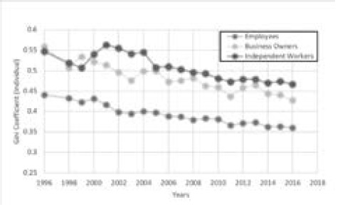
Figure 5:
Inequality by occupation in Mexico 1996-2016 (individual income)

Overall, the patters on these graphs indicate an increase on inequality when the unit of analysis is the household and a decrease of income inequality when the unit of analysis is the individual earner. As a measure of labor activity and unemployment, using income earners as a unit of analysis is convenient and necessary, but to estimate and understand the impact of policy changes on income inequality and on social welfare, it is the household the required unit of analysis. Estimating the average household income provides a more consistent and realistic value of income inequality, and it incorporates the complexity of a social structure like the family in the estimation.

THE INCOME-INEQUALITY RELATIONSHIP IN MEXICO AND THE AUGMENTED KUZNETS CURVE

After the examination of the data for inequality and income at the subnational level, it was evident that in Mexico exists a negative relationship between inequality (measured by Gini coefficients), and income. In both specifications: using individual income (earners only) or household income, the slope of the fitted line is negative. This supports the original Kuznets theory that inequality decreases at higher levels of income, when the transition to a more modern industry has been realized. Figure 6 shows scatter plots with trend lines showing that as income is higher, the Gini coefficient is lower, so inequality decreases.

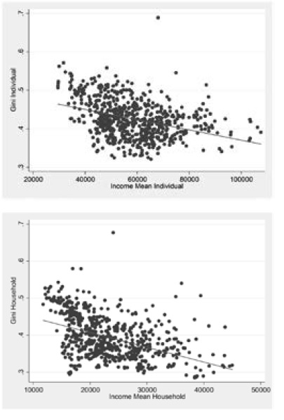
Figure 6:
Income-inequality relationship using individual and household income

Based on this analysis, there is no clear evidence to suggest the presence in Mexico of an Augmented Kuznets curve. This occurs when economies have specialized in more modern segments of the economy (such as technology and capital goods), with higher levels of income, but also reporting increments in the levels of inequality.

INCOME INEQUALITY IN MEXICO AFTER THE REFORMS OF 2014: AN INTERRUPTED TIME SERIES

After exploring the inequality patterns for the period of study, Gini coefficients per state per year were calculated and used to evaluate if inequality has increased since 2014. By modeling this change in the Mexican economy as an intervention and controlling for income, an Interrupted Time Series (ITS) design was introduced.

The regression model is the following:

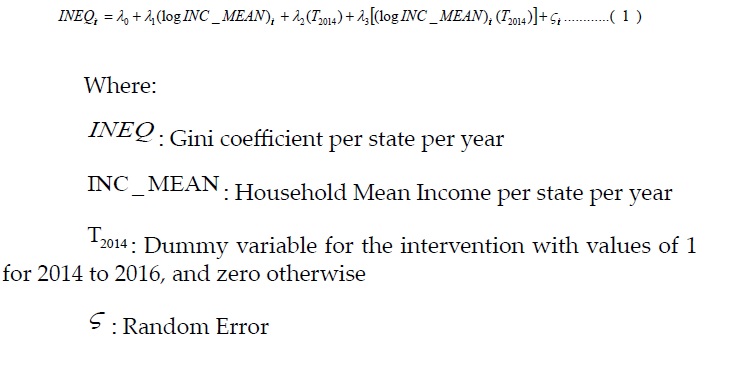
In this case, we are including an indicator variable to control for the new policy implementation and an interaction term to allow for a possible change in slope. The dependent variable is the Gini coefficient measured as an index with a range from 0 to 100 to avoid having very small coefficients, and to simplify their interpretation. The independent variables are household mean income in logarithmic form, an indicator variable to account for a change in the intercept due to the new policy, an interaction term between household mean income (in logarithmic form), and the time dummy variable. This variable will account for changes in the slope of the regression line.

The results are reported in Table 1, using four methods to estimate the regression. The first method is the Ordinary Least Square, hereafter the OLS Model, which estimates present problems of consistency and heterogeneity bias, but which are included as a baseline. The second model reported in Table 1 shows the coefficients for the Fixed Effects estimation, controlling for panel effects (states) and heteroskedasticity⁸. The third column reports the model obtained with Random Effects with robust standard errors, and the fourth and last column reports the estimates of the feasible GLS Model which addresses issues of autocorrelation and heteroskedasticity.

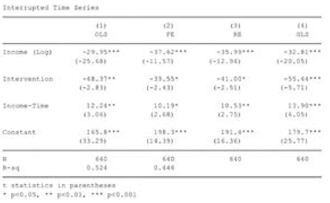
Table 1:
Interrupted time series with policy intervention in 2014

In the four models, the variable Income is statistically significant with a negative sign, showing that as income increases, inequality tends to decrease, supporting the Kuznets hypothesis after transition to an industrialized economy. In the case of the Intervention variable which measures the change in intercept of the regression line, and identifies the impact of changes in the policy, the variable is statistically significant at least at 5% level for the four models.

The interaction between income and the policy intervention, the Income-time variable, is statistically significant for the four models, providing evidence that suggests that there is a change in slope in the regression line after the intervention. The most robust of the four models is Model 2, estimated with Fixed Effects which controls for differences in the panels (states). The interpretation for the variables Intervention and Income-Time combined is that for those observations after the intervention, the impact of an increase in income has a more pronounced effect in inequality, but the effect is positive⁹.

Figure 7 reports the actual and the predicted Gini coefficients per state per year to show the change in trend after 2014. In Figure 8, a stylized version of the Interrupted Time Series is included, to represent the effect of the policy intervention in the predicted Gini coefficients, showing a change in the slope and on the intercept of the regression line once the intervention takes place in 2014¹⁰.

These are the graphical representation of what Table 1 is reporting, as the intervention is affecting the levels of inequality and the change in slope and direction, they seem to indicate that there is a significant change in the inequality levels in Mexico after the intervention, when controlling for income.

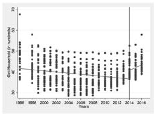
Figure 7:
Interrupted time series with Gini coefficients per state per year

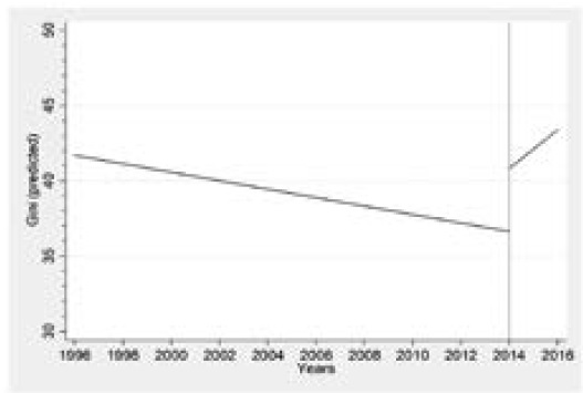
Figure 8:
An interrupted time series design, the effects of reforms on inequality in Mexico

CONCLUSIONS

After examining the data, there was evidence to suggest that the levels of inequality have increased for the period of study when the unit of analysis is the household. This could be explained by an increase in the number of dependents without income per household. These individuals could be dependent or unemployed. In the last ten years, Mexican unemployment rate increased in 2009 to 5% and stayed around that level until 2014. This increase may be explained in the context of the global recession of 2008-2009.

When the analysis of inequality is based on individuals, then the levels of inequality have a decreasing trend for the period of study. The Gini coefficient calculated with this data measures the differences in income among earners, ignoring those who reported zero income.

In the case of rural and urban sectors, household inequality maintains the general trend, with a decrease in the middle of the period and an increase in the last years of the period of study, with rural inequality having an overall increasing trend, closing the gap with the levels of inequality in the urban sector.

In the case of occupations, with inequality measured per individual earners, the trend is decreasing for the three most important occupational groups: Employees, Business Owners and Independent Workers. As expected, the group of employees reports the lowest levels of inequality, and the other two groups report higher inequality coefficients across the period.

From the policy perspective, this evidence suggests the need to evaluate the implementation of unemployment benefits, at least for a short period of time to mitigate the problems derived from exogenous macroeconomic events. Also, relevant policy to promote rural development should be revised and evaluated. Programs such as Procampo to stimulate investment in the agricultural sector, as well as programs to regulate ownership of the land must be examined and audited to know their scope and their actual benefits across the country.

In the case of the relationship between inequality and income, known as the Kuznets hypothesis, there is evidence in the Mexican context of a decline in inequality as income increases. This analysis was based on household data and individual data. Both measures showed the same pattern. The Kuznets curve explains that after the transition to an industry driven economy, inequality decreases as the benefits of modernization spread across society.

This transition is not new in Mexico, so the negative relationship between income and inequality was expected. However, more advances economies will manifest a second Kuznets curve (the Augmented Kuznets hypothesis) when a new economic transition is present, and economies move to more advanced and technological intensive industries. In Mexico, there is no evidence to suggest the presence of an increase in inequality and income simultaneously.

The policy implication in this case must be to focus in programs that encourage investment on new industries, with new technologies as an engine of change. The idea is that even if inequality increases even more, an increase in income percapita will benefit society and eventually the Kuznets curve will shift to a new cycle of decreasing inequality with higher levels of income.

In the case of the effect of new regulations on the levels of inequality in Mexico, evidence was found to suggest that there is a change in the pattern of inequality after 2014, when the new federal regulations were on effect. The Interrupted Time Series analysis showed a clear change in the slope of the regression before and after the policy intervention. By using the 32 Mexican States as panels with 20 years of data, the regression shows that before 2014, the slope of the predicted values is negative.

This means than when controlling for income, the inequality reveals a decreasing trend. When the intervention was effective (in 2014), the new predicted line shows a similar intercept, but the slope is now positive, with an ascending trend, implying that inequality increases as time progresses when controlling for income.

The four models prepared using OLS, Fixed Effects, Random Effects and GLS report consistent results, with a negative and significant coefficient for Income, a negative and significant coefficient for the Intervention dummy variable, and a positive and significant coefficient for the interaction term between income and the dummy variable, Income-Time. These effects however can be temporal, and may change once more years are added after the intervention.

As the current policy reforms appear to have an impact on income inequality, the Federal Government should evaluate if the implemented changes have the expected effects.

The recommendation is to create an autonomous entity, working directly with Congress, to examine the preliminary results of the Tax Reform and to measure if the benefits outweigh the costs. It is possible that this is a short term effect which will change once the reforms are completely in effect, but there is enough evidence to warrant a continue assessment and revision of the policy.

References

1 BRUSSOLO, M. (2007). Agriculture in Mexico: The Agrarian Reform and the Challenges of Free Trade, University of Texas of Dallas (unpublished).

2 BRUSSOLO, M. (2011). The Kuznets’ Hypothesis Revisited: Exploring Mexican Inequality at the Sub-National Level, Ph.D. dissertation.

3 CONCEIÇÃO, P. & GALBRAITH, J.K. (2001). Toward an Augmented Kuznets Hypothesis. Inequality and Industrial Change: A Global View, Cambridge, Cambridge University Press.

4 FOSTER, J.E. (2006). Inequality Measurement, The Elgar Companion to Development Studies, Cheltenham, U.K. and Northampton, Mass., Elgar, pp. 275-281.

5 GINI, C. (1921). “Measurement of Inequality of Incomes”, The Economic Journal, 31, pp. 124-126.

6 INEGI (2001). Documento metodológico de la Encuesta Nacional de Empleo Urbano. http://www.inegi.org.mx/prod_serv/contenidos/espanol/biblioteca/default.aspaccion=1&upc=702825000017&s=est &c=10735

7 INEGI (2005). Encuesta Nacional de Ocupación y Empleo 2005, una nueva encuesta para México.http://www.inegi.org.mx/est/contenidos/espanol/metodologias/encuestas/hogares/sm_enoe.pdf.

8 INEGI (2007). Cómo se hace la ENOE. Métodos y procedimientos.http://www.inegi.org.mx/est/contenidos/espanol/metodologias/enoe/ENOE_como_se_hace_la_ENOE1.pdf.

9 INEGI (2008). Homologación de la serie de indicadores estratégicos ENE-ENOE. Documento técnico. http://www.inegi.org.mx/est/contenidos/espanol/metodologias/encuestas/hogares/sm_laboral.pdf.

10 INEGI (2009a). Consulta de microdatos de la Encuesta Nacional de Empleo (ENE) y documentos asociados.http://www.inegi.org.mx/inegi/default.aspx?s=est&c=10653&e=&i=.

11 INEGI (2016). Consulta de microdatos de la Encuesta Nacional de Ocupación y Empleo (ENOE) y documentos asociados.http://www.inegi.org.mx/inegi/default.aspx?s=est&c=10781&e=&i=.

12 JACOBS, D. (2008). Fixed Effects, Autocorrelation Heteros-kedasticity. The Stata Listserver. http://www.stata.com/statalist/archive/2008-08/msg00953.html.

13 KUZNETS, S. (1955, 3). “Economic Growth and Income Inequality”, American Economic Review, 45 (1-24), pp. 1-28.

14 LEVINSON, B.A. (2014). “Education Reform Sparks Teacher Protest in Mexico”, Phi Delta Kappa, 95(8), pp. 48-51.

15 SECRETARÍA DE HACIENDA Y CRÉDITO PÚBLICO, S.A.T. (2016). Cuadro histórico de salarios mínimos (1982-2016).http://www.sat.gob.mx/informacion_fiscal/tablas_indicadores/Paginas/ inpc_2014.aspx

16 SEN, A. (1973). On Economic Inequality, N. York, Norton. STOCK, J.H. & WATSON, M.W. (2006). HeteroskedasticityRobust Standard Errors for Fixed Effects Panel Data Regression, NBER Technical Working Paper No. 32.

Notes