Articles
A conditional heteroscedastic VaR approach with alternative distributions
Un enfoque del VaR heterocedástico condicional con distribuciones alternativas
A conditional heteroscedastic VaR approach with alternative distributions
EconoQuantum, vol. 17, no. 2, pp. 81-98, 2020
Universidad de Guadalajara
Received: 09 August 2018
Accepted: 31 October 2019
Abstract:
Objective: The purpose of this paper is to explore different distributions in conditional Value at Risk (VaR) modeling as an option in the Mexican market. Methodology: We estimate a GARCH model under the Gaussian, Normal Inverse Gaussian, Skew Generalized t and the Stable distribution assumption, then we implement the model in predicting one-day ahead VaR and finally we examine the performance among the four VaR models during a period of high volatility.
Results: The backtesting result confirms that the stable-VaR approach outperforms the other models in the VaR’s prediction at 99% confidence level.
Limitations: Although the VaR is a widely used risk measure is not a coherent risk measure, for this reason, a natural extension of our work should be to estimate the expected shortfall and this may produce different insights.
Conclusions: Our findings reveal that models that consider some empirical characteristic of financial returns such as leptokurtic, volatility clustering and asymmetry improve the VaR predicting capacity. This finding is important in the search more robust approaches for VaR estimates.
Keywords: VaR+ GARCH+ Stable distribution+ Generalized Skew t distribution+ Normal Inverse Gaussian distribution+ G17+ C22+ C53.
Resumen:
Objetivo: El propósito de este trabajo es explorar diferentes distribuciones en la estimación del Valor en Riesgo (VaR) como una opción en el mercado mexicano.
Metodología: Estimamos un modelo GARCH bajo la hipótesis de las distribuciones Gaussiana, Normal Inversa Gaussiana, t-student Sesgada Generalizada y Estable. Implementamos este modelo para predecir los VaR a un día y finalmente examinamos el desempeño de estos cuatro modelos VaR durante una período de alta volatilidad.
Resultados: El resultado del backtesting confirma que el VaR estable a un nivel de confianza del 99% supera a los otros modelos en la predicción del VaR. Limitaciones: Aunque el VaR es una medida de riesgo ampliamente utilizada, no es una medida de riesgo coherente, por esta razón, una extensión natural de nuestra investigación sería estimar el Valor en Riesgo Condicional (CVaR) lo cual podría generar diferentes resultados.
Conclusiones: Nuestros hallazgos revelan que los modelos que consideran algunas características empíricas de los rendimientos financieros, tales como leptocurtosis, agrupamiento de volatilidad y asimetría, mejoran la capacidad de predicción del VaR. Lo anterior es importante en la búsqueda de enfoques más precisos y eficientes en la estimación de VaR.
Palabras clave: VaR, GARCH, distribución estable, distribución t-student sesgada generalizada, distribución normal inversa gaussiana, G17, C22, C53.
Introduction
The first objective of the present paper is to different distributions in conditional Value at Risk (VaR) modeling as an option in the Mexican market. The interest in stable distributions has been increasing since the seminal work by Mandelbrot (1963) and Fama (1965) led them to the conclusion that marginal distributions of financial data exhibit skewness and leptokurtosis.
Empirical evidence reveals that stable distributions capture the leptokurtic nature of financial data (Fama, 1965a; Mandelbrodt, 1963, 1967; McCulloch, 1986; Mittnik, Paolella, & Rachev, 2000; Nolan, 2014; Panorska, Mittnik, & Rachev, 1995) and they satisfy the Generalized Central Limit Theorem which state that the only possible non- trivial limit of normalized sums of independent identically distributed (i.i.d) random variables is stable.
In addition, some empirical research works that assumed the stable distribution hypothesis in the optimal portfolio problem are Rachev & Han (2000); Ortobelli, Huber, & Schwartz (2002) that analyzed and compared the performance of the stable distribution assumption in portfolio theory considering the S&P500, DAX30 and CAC40 indexes. In the same line, Climent, Venegas & Ortiz (2015) studied the optimal portfolio problem under the stable hypothesis and compared its performance with a Gaussian optimal portfolio, their results showed that the stable optimal portfolio has higher re- turns and lower risk.
Dias Curto, Castro Pinto, & Nuno Tavares (2009) examined alternative conditional distributions (Normal, t-student and stable) for the DJIA, DAX and PSI20 indexes considering an AR-GARCH model, their results show that the stable-GARCH model describes better the stock returns’ volatility. Similarly, Mohammadi (2017) analyzed the volatility predictive performance of the stable-GARCH and stable power-GARCH models and applied this method for predicting future values of the S&P500 stock market.
Khindanova, Rachev, & Schwartz (2001) applied stable distribution in VaR modeling the forecast evaluation shows that stable VaR outperforms the normal modeling. Serrano & Mata (2018) compared the VaR estimation under the stable and normal GARCH approach before, during and after a crisis period the results provide evidence that the stable model provides better VaR estimates the normal one during a crisis period but in tranquility periods, it overestimates the potential losses.
The other distributions considered as an alternative for VaR modeling are the Skew Generalized t (GST) and Normal Inverse Gaussian (NIG) distributions. We chose the family of GST distributions originally introduced by Theodossiou (1998) as a skew extension of the generalized t (GT) distribution because it provides a flexible tool for modeling data exhibiting diverse levels of tail thickness, skewness, and peakedness around the location. Many of the widely used distributions such as t-student, normal, Hansen’s skew t, exponential power, and skew exponential power (SEP) distributions are included as limiting or special cases in the GST family.
The GST distribution has been widely used for modeling financial data, for example, Bali & Theodossiou (2007) computed the VaR considering ten different specifications of the GARCH model based on the GST distribution, the results indicate that the TS-GARCH and EGARCH models have the best overall performance in terms of VaR accuracy.
More recently, Corlu, Meterelliyoz & Tiniç (2016) analyzed the suitability of GST, NIG and generalized lambda (GLD) distributions among others to describe stylized characteristic on the equity index returns of twenty different countries and evaluated the models using the in-sample VaR failure rates, the results suggest that the GLD distribution is the best alternative, although this paper is focused only on the unconditional distribution of equity returns.
On the other hand, the NIG distribution is a versatile univariate probability distribution that can capture, by its parameters, the stylized facts of heavy tails, skewness and kurtosis of asset yields (Protassov, 2004). Usually the literature defines the probability density function as Barndorff-Nielsen (1977) and Prause (1999), so NIG is defined as the mean-variance mix between a normal random variable and a generalized inverse Gaussian random variable (GIG).
Applications of the NIG distribution in finance have been found in several studies, for example, Barndorff-Nielsen (1977); Bølviken & Benth (2000) studied if the NIG model is suitable for VaR evaluations in the Norwegian case; Corlu et al. (2016) analyzed the suitability of GST, NIG and generalized lambda (GLD) distributions among others to describe stylized characteristic on the equity index returns of twenty different countries.
However, the focus in the literature has been on portfolio optimization, volatility predictive performance and VaR modeling for developed stock markets. To our knowledge, there are no studies that apply a stable-GARCH model in VaR modeling in the Mexican market and compare its predictive performance during a crisis period with the one based on the GARCH model under the GST, normal and NIG hypotheses, respectively.
The rest of the paper is organized as follows: The second section presents details related to the probability density functions, the methodologies of the GARCH models, the measurement of VaR and the backtesting methodology. The third section describes the data and contains the empirical results. The fourth section compares the out-of-sample empirical results. The fifth section concludes the paper.
Methodology
Value at Risk (VaR)
VaR methodology is commonly used for measuring market risk; it is a suitable measurement since regulators accept this quantity as a basis for setting capital requirements for market risk exposure.
A VaR measure is the maximum loss on a period of time (τ) at a specific confidence level (1 - q). More formally, VaR is defined as:
where X represents the portfolio’s returns.
This definition can be rewritten in terms of the probability distribution of portfolio value returns as follows:
where is the inverse cumulative distribution function of portfolio returns in one period.
VaR estimates can be obtained via parametric approach, historical simulation and Monte Carlo simulation.
Probability density functions
The development of more robust approaches for VaR estimates is crucial. In this paper, we apply probability and time series theory to improve estimations of appropriate underlying distributions, to capture fat tails and volatility of conditional return distributions; and as a result, improve the estimation of VaR.
In this work, we introduce three families of distributions: Hansen’s skew t distribution (Hansen-GST), NIG and stable distribution, which can capture the kurtosis and skewness of financial returns (Rachev & Han, 2000; Mittnik et al. 2000).
Hansen’s skew t distribution (Hansen-GST). Hansen (1994) proposed a different parametric approach to modeling the conditional density of the normalized error. His suggestion is to select a distribution which depends upon a low-dimensional parameter vector, and then let this parameter vector vary as a function of the conditional variables.
Definition. Hansen-GST distribution is a simple skewed generalization of t-Student density. The probability density function is defined as follows:
where 2 < η < ∞, - 1 < λ < 1. The constants a, b and c are given by , and .
The parameter η controls the tail thickness and λ controls the skewness. When η → ∞, it is reduced to skewed normal distribution. When λ = 0, it is reduced to Student’s t distribution. Figure 1 gives the probability density function of Hansen-GST with different parameters. We can see that the smaller η is, the fatter the tail is.
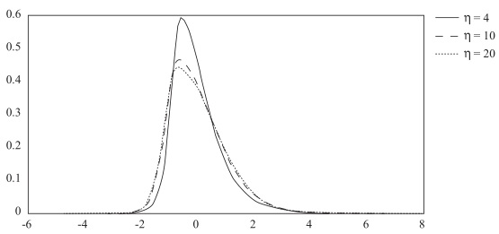
Figure 1
Hansen’s skew t distribution with λ=0.5 and η=4, 10, 20
If a random variable Z follows a standard Hansen-GST distribution with parameter η and λ, we write it as Z + GST(η,λ).
Normal Inverse Gaussian distribution (NIG). The NIG distribution is a specific case of the generalized hyperbolic distribution with λ = −1/2.
Definition. A random variable X follows a NIG distribution with parameters λ = -1/2, X ≥ 0 and Ψ ≥ 0 if the probability density function is
where α, δ ≥ 0 and μ, β ∈ ℝ such that β ∈ [-α,α] and kλ is the third order modified Bessel function. The parameter β represents the asymmetry, a the heaviness of the tails, λ captures the form of the distribution, μ is a location parameter and δ measures the dispersion (Corlu et al., 2016).
Stable distribution. The stable distribution is capable of capturing skewness and heavy tails and having many intriguing mathematical properties (Devroye & James, 2014; Fofack, & Nolan, 1999; Zolotarev, 1989). The class was characterized by Paul Lévy in his study of sums of independent identically distributed terms in the 1920’s.
Stable distributions do not have mathematical expressions for their probability density (PDF) and cumulative distribution (CDF) functions, instead they are described by their characteristic function (CF).
Definition. A characteristic function of a stable random variable X is defined as follows:
where 0 < α ≤ 2 is the index of stability or characteristic exponent, -1 ≤ β ≤ 1 is the skewness parameter, γ ≥ 0 is the scale parameter, and δ ∈ R is the location parameter.
If a stable random variable X follows a stable distribution, we write it as X ~ S (α, β, γ, δ). See Figure 2 for plots of stable densities.

Figure 2
Stable densities S (α, β, γ, δ)
Since we cannot get closed form of PDF and CDF for stable distributions (except that α = 2), we calculate them numerically (Mittnik, Doganoglu, & Chenyao, 1999; Nolan, 1997).
Goodness of fit. We use the Kolmogorov-Smirnov (KS) and Anderson-Darling (AD) statistics to compare the goodness-of-fit of the distributions of interest. The KS test statistic computes the difference between the fitted cumulative distribution function F(x) and the empirical cumulative distribution function as follows: .
The AD test statistic computes the weighted average of the squared differences as follows: , where the weights are chosen in such way that the discrepancies in the tails are emphasized.
GARCH models
Volatility plays an important role in financial models of pricing and hedging. For this reason finding the conditional distributions on which their estimates of this are more efficient is crucial. The traditional GARCH-normal model fails to capture the non-normal characteristics of financial returns. In this paper, we use three flexible distributions to describe the volatility of the stock returns characterized by leptokurtosis and skewness.
Empirical studies support that the GARCH (1, 1) model works well for financial data (Bali, & Theodossiou, 2007; Liu, & Brorsen, 1995; Panorska, Mittnik, & Rachev, 1995). It is important to mention that Starica (2003) shows that the GARCH (1,1) model has a poor volatility forecasting over long horizons, although at the same time he states that its model provides a precise estimation in a sample size of 2000 observations approximately.
GARCH (1, 1) model with stable distribution (stable-GARCH). Following Panorska, Mittnik, & Rachev (1995) and Naka & Oral (2013) we used the GARCH model proposed by Taylor (1986) and Schwert (1989). Since stable distributions do not have the second absolute expectation (except when α = 2), the conditional variance is expressed in terms of the conditional standard deviation as follows:
where Rt is the series of individual stock return at time t, μt and σt are, respectively, the conditional mean and conditional standard deviation of Rt, and zt are i.i.d. standardized stable random variables, zt ~ S(α, β, 1, 0) with 1 < α < 2 .
To estimate the parameters in (6), we use the Maximum Likelihood Estimation (MLE) method1, where the PDFs of zt were approximated using the computer program STABLE.2
Hansen-GST GARCH model. We consider the Hansen-GST distribution as the innovation in the GARCH model to describe the asymmetry and fat-tail property. The model is set up as follows.
Individual stock return is modeled as
To estimate the parameters in (7), we use the MLE method, where the pdfs of zt are approximated using the approach proposed by Hansen (1994).
NIG and Gaussian GARCH model. We consider the NIG and the Gaussian distributions as the innovation in the GARCH model. Individual stock return is modeled as (7) with c = 0. To estimate the parameters of the NIG distribution, we use MLE.
Estimating VaR
VaR estimation is realized by Monte Carlo simulation (Embrechts, McNeil & Frey, 2005; Glasserman, 2003) considering a heteroscedastic VaR model on the basis of the stable distribution, Hansen-GST, NIG and normal distribution. We simulated 10,000 realizations of the series of individual stock returns at time t and measure VaR as the negative of the q-th quantile of the simulated return’s distribution.
Backtesting
Since financial institutions have the freedom to specify their own model to compute their VaR, the procedure to backtesting becomes extremely important for regulators to assess the quality of the models.
We evaluate and compare the performance for distributions-based heteroscedastic VaR models based on the Kupiec Unconditional Coverage (UC) test (1995) and the Christoffersen Conditional Coverage (CC) test (1998).
The Kupiec Unconditional coverage test (UC). Suppose we use the most recent k historical data to forecast the current VaR, define the indicator for VaR violations as follows:
where H are the historical returns and s = 1, ..., k.
The Kupiec likelihood ratio test (Kupiec, 1995) tests the null hypothesis:
i.e. it tests whether the expected proportion of violations is equal to α.
The likelihood ratio test statistic is given by:
where N is the sample size, n is the number of violations and p = n/N is the percentage of violations. This test follows an asymptotic chi-square distribution with one degree of freedom.
The Christoffersen Conditional Coverage test (CC). The Conditional Coverage test (Christoffersen, 1998) requires a correct unconditional coverage and furthermore, it ensures that the result series is i.i.d. This statistic test follows an asymptotic chi-square distribution with two degrees of freedom and is given by:
where nij is the number of observations with value i followed by j, and πij = Pr(Is (α) = j|Is-1 (α) i).
Empirical results
Data and descriptive statistics
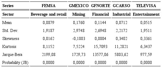
For the empirical analysis, five assets with a different trading volume from five different industries listed on the Mexican Stock Exchange (BMV) have been chosen. These assets correspond to the following companies: Fomento Economico Mexicano, S.A.B. de C.V. (FEMSA) is a company that through its subsidiaries produces, distributes and markets non-alcoholic beverages throughout Latin America as part of the Coca-Cola system. The Company owns and operates convenience stores in Mexico and Colombia and holds a stake in Heineken; Grupo Carso (GCARSO) one of the most important conglomerates in Latin America, the company controls and operates companies in the industrial, commercial, infrastructure and construction sectors; Grupo Mexico S.A.B. de C.V. (GMEXICO) holds concessions to operate the Pacifico-Norte and Chihuahua-Pacifico Railroad lines. Grupo Mexico, through subsidiaries, operates open-pit copper mines, underground mines, a coal mine, copper smelters, a rod mill facility, and a precious metals refinery; Grupo Financiero Banorte S.A.B. de C.V. (GFNORTE) is a financial institution in Mexico. The Company offers banking services, premium banking, whole- sale banking, leasing and factoring, warehousing, insurance, pensions and retirement savings; and Grupo Televisa, S.A.B., (TELEVISA), operates media and entertainment businesses in the Spanish speaking world. The Company has interests in television production and broadcasting, programming, direct-to-home satellite services, publishing and publishing distribution, cable television, radio production, show business, feature films and Internet portals.
We estimate the VaR of these five stocks (based on daily closing prices) over the period January 2, 2002 to December 31, 2009, about 2018 observations for each stock. The reference currency used is the Mexican peso and the asset returns are logarithmic returns. The series plot of the 5 stocks returns are shown in Figure 3.
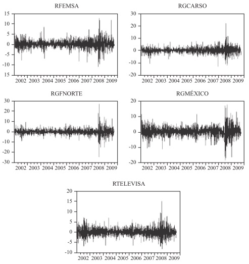
Figure 3
Daily returns (%)
Descriptive statistics of daily returns are presented in Table 1. Based on the skewness and kurtosis we observed that the data are asymmetric and have thicker tails than the normal distribution. In addition, the Jarque-Bera statistic is large and statistically significant, thereby implying that the assumption of normality is rejected.
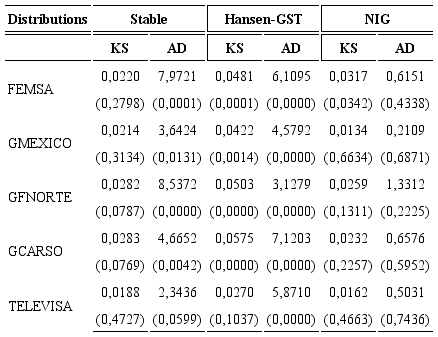
Goodness of fit
We use the KS and AD statistics to compare the goodness-of-fit of the distributions of interest. Table 2 presents the hypothesis test KS and AD to verify if the time series of the daily returns follow the proposed probability distribution, the p-value is reported in brackets. The null hypothesis is that the observed data originates from the hypothesized distribution and is rejected if the p-value is lower than α = 1%. It can be seen that each time series is adjusted to some probability distribution under a significance level of 1%.
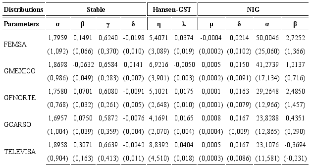
To estimate the different parameters of the probability density functions that have been proposed in this work, we use the MLE method. Table 3 shows these estimators, standard errors are in brackets.
Estimating GARCH models
Tables 4 and 5 present the maximum likelihood estimation for the GARCH models assuming the alternative distribution functions, standard errors are in brackets.
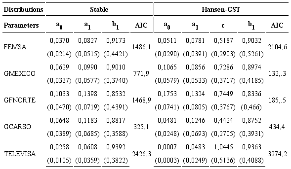
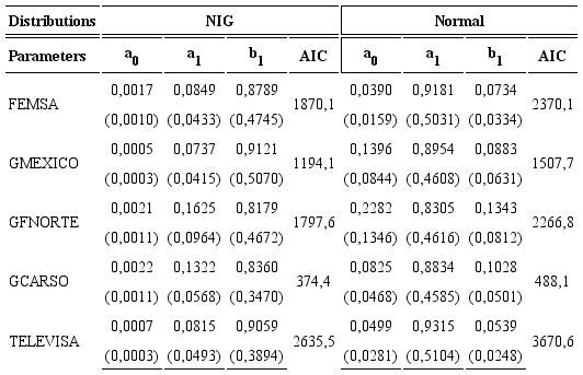
We can observe from Tables 4 and 5 that the sum of the parameters are less than one, ensuring the conditions for stationarity, in addition, for the Hansen-GST GARCH model the asymmetric coefficients are significant, indicating the presence of asymmetric leverage volatility effects. Finally, the Akaike Information Criterion (AIC) indicates that the GARCH stable is the model that better captures the dynamics of the returns series; it is followed by the NIG GARCH model, next to the Hansen-GST and the normal GARCH models.
VaR estimates
VaR estimation is realized by Monte Carlo simulation based on 10,000 realizations of the series of individual stock. Table 6 provides the one-day ahead estimates of VaR for each returns, at 95% and 99% confidence levels.
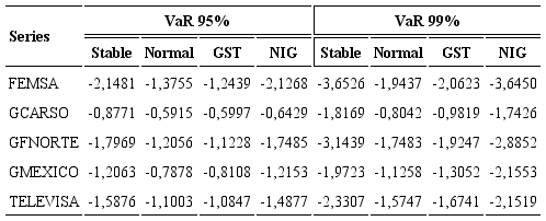
As observed in Table 6, except for GMEXICO, the stable-VaR estimates at 95% and 99% confidence levels are higher than the normal, NIG and Hansen-GST VaR estimates, i.e., the stable VaR measurements provide more conservative53 VaR estimates of potential losses. On the contrary, the normal distribution produces the lowest VaR estimates at 99% among the four VaR models.
Evaluation of performance of heteroscedastic VaR models
We evaluated the performance of the heteroskedastic conditional Stable, Hansen-GST, NIG and Normal VaR models by computing the out-of-sample forecasts based on the Kupiec UC test and the Christoffersen CC test. The predicted one-day-ahead VaR is based on a rolling window out-of- sample procedure. The window size is fixed at 502 observations, i.e., we used the most recent two years of historical data to estimate the current VaR.
Tables 7 and 8 provide the backtesting results of VaR. The symbol “X” is used in the table to denote VaR models which pass the unconditional coverage test. Asterisk “*” and minus “-” signs indicate that the conditional coverage test is rejected at the 1% significance level as a result of overestimation and underestimation of the realized VaR, respectively. Models that satisfy the hypothesis of correct conditional coverage are accepted as well-specified VaR models.
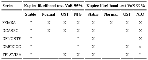
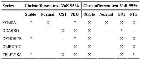
From Tables 7 and 8 we can see that the NIG-VaR model provides correct unconditional and conditional coverage for three of the five series at 95% confidence level.
Besides the normal VaR approach tends to underestimate real market risk. At 99% confidence level the stable-VaR estimates passed both tests, i.e the stable-VaR approach does very well in predicting critical loss at this confidence level. In addition, the GST and NIG also show good results, four of the five series passed the CC test; in contrast, the conditional normal VaR measurements significantly underestimate the potential losses.
Conclusions
In this paper, we estimated a GARCH model assuming three flexible distributions to describe the volatility of the stock returns characterized by leptokurtosis and skewness. We then implemented it in predicting one-day ahead VaRs and compared it with that of the GARCH-normal VaR model.
The empirical results suggest that the forecasted VaR obtained using the stable distribution provides the most accurate out-of-sample forecasts a 99% confidence level, i.e., our model improves the performance VaR measurements at this level with the stable distributional assumption. In contrast, this approach overestimates the VaR a 95% confidence level.
Besides the VaR models based on GST and NIG distributions perform relatively better than the normal distribution at low confidence level and have a satisfactory performance at 99% confidence level.
Our findings reveal that models that consider some empirical characteristic of financial returns such as leptokurtic, volatility clustering and asymmetry improve the VaR predicting capacity. This finding is important in the search for more robust approaches for VaR estimates.
Additionally, the stable distribution appears to be the most appropriate alternative in VaR modeling a 99% confidence level in the Mexican financial market. However, additional research is needed. Multivariate stable distributions will be employed in future research to describe and examine portfolios behavior during financial crises.
References
Bali, T.G., & Theodossiou, P. (2007). A conditional-SGT-VaR approach with alternative GARCH models. Annals of Operations Research (151), 241-267. DOI: https://doi.org/10.1007/s10479-006-0118-4
Bølviken, E., & Benth, F.E. (2000). Quantification of risk in Norwegian stocks via the normal inverse Gaussian distribution. Proceedings of the AFIR 2000 Colloquium, Tromso, Norway (pp. 87-98). Retrieved from http://www.actuaries.org/AFIR/Colloquia/Tromsoe/Bolviken_Benth.pdf
Christoffersen, P.F. (1998). Evaluating interval forecasts. International Economic Review, 39 (4), 841-862.
Climent Hernández, J.A., Venegas Martínez, F., & Ortiz Arango, F. (2015). Portafolio óptimo y productos estructurados en mercados a-estables un enfoque de minimización de riesgo. Revista Nicolaita de Estudios Económicos, 10 (2), 81-110.
Corlu, G., Meterelliyoz, M., & Tiniç, M. (2016). Empirical distributions of daily equity index returns: A comparison. Expert Systems with Applications, 54, 170-192. DOI: https://doi.org/10.1016/j.eswa.2015.12.048
Devroye, L., & James, L. (2014). On simulation and properties of the stable law. Statistical Methods & Applications, 23 (3), 307-343. DOI: https://doi.org/10.1007/s10260-014-0260-0
Dias Curto, J., Castro Pinto, J., & Nuno Tavares, G. (2009). Modeling stock markets’ volatility using GARCH models with normal, student’s t and stable paretian distributions. Statistical Papers, 50 (2), 311-321. DOI: https://doi.org/10.1007/s00362-007-0080-5
Fama, E.F. (1965a). Portfolio analysis in a stable paretian market. Management Science, 11 (3), 404-419. DOI: https://doi.org/10.1287/mnsc.11.3.404
Fama, E. F. (1965b). The behavior of stock-market prices. The Journal of Business, 38 (1), 34-105.
Fofack, H., & Nolan, J.P. (1999). Tail behavior, modes and other characteristics of stable distributions. Extremes, 2, 39-58. DOI: https://doi.org/10.1023/A:1009908026279
Hansen, B. E. (1994). Autoregressive conditional density estimation. International Economic Review, 35 (3), 705-730.
Khindanova, I., Rachev, S., & Schwartz, E. (2001). Stable modeling of value at risk. Mathematical and Computer Modelling, 34, 1223-1259.
Kupiec, P.H. (1995). Techniques for verifying the accuracy of risk measurement models. The Journal of Derivatives, 3 (2) 73-84. DOI: https://doi.org/10.3905/jod.1995.407942
Liu, S.M., & Brorsen, B.W. (1995). Maximum likelihood estimation of a GARCH- stable model. Journal of Applied Economics, 10, 273-285.
Mandelbrot, B.B. (1963). The variation of certain speculative prices. The Journal of Business, 36, 394-419.
Mandelbrodt, B.B. (1967). The variation of some other speculative prices. The Journal of Business, 40, 394-419.
McCulloch, J.H. (1986). Simple consistent estimators of stable distribution parameters. Communications in Statistics - Simulation and Computation, 15 (4), 1109-1136. DOI: https://doi.org/10.1080/03610918608812563
Mittnik, S., Doganoglu, T., & Chenyao, D. (1999). Computing the probability density function of the stable Paretian distribution. Mathematical and Computer Modelling, 29 (10/12), 235-240. DOI: https://doi.org/10.1016/S0895-7177(99)00106-5
Mittnik, S., Paolella, M.S., & Rachev, S.T. (2000). Diagnosing and treating the fat tails in financial returns data. Journal of Empirical Finance, 7 (3/4), 389-416. DOI: https://doi.org/10.1016/S0927-5398(00)00019-0
Mohammadi, M. (2017). Prediction of α -stable GARCH and ARMA-GARCH-M models. Journal of Forecasting, 36 (7), 859-866. DOI: https://doi.org/10.1002/for.2477
Naka, A., & Oral, E. (2013). Stock return volatility and trading volume relationships captured with stable paretian GARCH and threshold GARCH models. Journal of Business & Economic Research, 11 (1), 47-53.
Nolan, J.P. (2001). Maximum likelihood estimation and diagnostics for stable distributions. In O.E. Barndorff-Nielsen, S.I. Resnick, & T. Mikosch (Eds.), Lévy Processes (pp. 379-400). Boston: Birkhäuser Boston. DOI: https://doi.org/10.1007/978-1-4612-0197-7_17
Nolan, J.P. (2014). Financial modeling with heavy-tailed stable distributions. Wiley Interdisciplinary Reviews: Computational Statistics, 6 (1), 45-55. DOI: https://doi.org/10.1002/wics.1286
Ortobelli, S., Huber, I., & Schwartz, E. (2002). Portfolio selection with stable distributed returns. Mathematical Methods of Operations Research, 55 (2), 265-300. DOI: https://doi.org/10.1007/s001860200182
Panorska, A., Mittnik, S., & Rachev, S.T. (1995). Stable GARCH models for financial time series. Applied Mathematics Letters, 8 (5), 33-37.
Rachev, S., & Han, S. (2000). Portfolio management with stable distributions. Mathematical Methods of Operation Research, 51, 341-352.
Schwert, G.W. (1989). Why does stock market volatility change over time? The Journal of Finance, 44 (5), 1115-1153.
Serrano Bautista, R., & Mata Mata, L. (2018). Valor en riesgo mediante un modelo heterocedástico condicional α-estable. Revista Mexicana de Economía y Finanzas, 13 (1), 1-25. DOI: https://doi.org/10.21919/remef.v13i1.257
Starica, C. (2003, diciembre). Is GARCH (1,1) as good a model as the accolades of the nobel prize would imply? (pp. 1-50). Retrieved from http://www.math.kth.se/matstat/seminarier/reports/M-exjobb10/100408.pdf
Theodossiou, P. (1998). Financial data and the skewed generalized T distribution. Management Science, 44 (12), 1650-1651.
Zolotarev, V.M. (1989). One-Dimensional stable distributions. Bulletin of the American Mathematical Society, 20 (2), 270-277.
Notes