Artigos
Proposition of credit risk forecasting models for small and medium enterprises through logistic regression
Proposição de modelos de previsão de risco de crédito para pequenas e médias empresaspor meio da Regressão Logística
Proposition of credit risk forecasting models for small and medium enterprises through logistic regression
Gestão & Regionalidade, vol. 38, núm. 113, pp. 219-240, 2022
Universidade Municipal de São Caetano do Sul

Esta obra está bajo una Licencia Creative Commons Atribución-NoComercial-SinDerivar 4.0 Internacional.
Recepción: 06 Abril 2020
Aprobación: 05 Abril 2021
Abstract: The search for standards that contribute to the prediction of risk is growing in organizations. The use of credit scoring models seeks to assist the credit analyst in making decisions. This work aims to develop methodological procedures, to structure and improve credit scoring models aimed at the analysis of small and medium-sized companies. With the use of the statistical technique of logistic regression, through the improvements developed in the methodological procedures, such as division of the database into classes according to the companies' framework, it was possible to develop 5 credit scoring models, one model for each class of companies and another for the general database. The models were directed to entities that promote and grant credit to small and medium-sized companies. The accuracy of the models showed significant percentages for the database with non-accounting and non-auditable variables, reaching satisfactory percentages.
Keywords: credit scoring, small and medium companies, logistic regression.
Resumo: A busca por padrões que contribuam na predição de risco, é crescente nas organizações. A utilização de modelos de credit scoring busca auxiliar o analista de crédito na tomada de decisão. Este trabalho objetiva elaborar procedimentos metodológicos, para estruturar e melhorar os modelos de credit scoring direcionados a análise de pequenas e médias empresas. Com a utilização da técnica estatística da regressão logística, por meio das melhorias elaboradas nos procedimentos metodológicos, como exemplo: divisão da base de dados em classes conforme enquadramento das empresas, foi possível o desenvolvimento de 5 modelos de credit scoring, sendo um modelo para cada classe de empresas e outro para a base geral de dados. Os modelos foram direcionados às entidades de fomento e concessão de crédito para pequenas e médias empresas. As acurácias dos modelos apresentaram percentuais expressivos para base de dados com variáveis não contábeis e não auditáveis, atingindo percentuais satisfatórios.
Palavras-chave: credit scoring, pequenas e médias empresas, regressão logística.
1 Introduction
Factors such as the increased degree of economic stability, the emergence of new products and services, and inflation control, contribute to the expansion of the consumer market (Ventura, 2010). This inclusion of people and companies in the Brazilian domestic market repositions credit analysis and its degree of importance since companies choose to market their products and services on credit terms, requiring evaluation criteria at the time of granting, since the risk of default is included in the sales process.
Risk assessment aims to improve the quality of a customer portfolio, favoring a healthy sale and avoiding as much as possible the loss of values, on credits provided in a wrong way or to customers who generate losses to the business. Companies that have a good assessment take advantage over their competitors (GOUVÊA; GONÇALVES, 2007).
One of the main informational bases is accounting, which must have a reliability of the information presented and be relevant so that the result of the concession analysis is useful. Bruni (2010) argues that much of the information worked out in the financial sector is recorded and stored in accounting.
Historically, small businesses face difficulties in accessing financing due to a lack of credible information, and sometimes do not have audited and certified financial statements regularly (BERGER; COWAN; FRAME, 2011).
Institutions that work focused on small and medium enterprises (SMEs) share the dilemma described by Berger, Cowan, and Frame (2011) and Berti (2012), regarding the credibility and auditing of accounting information, using other information sources for credit analysis (variables). Credit modeling presents itself as a support tool for analysts, however, there are few studies on credit modeling for small and medium-sized companies, highlighting the importance of these companies in the economies of countries around the world (LI; NISKANEN; KOLEHMAINEN, 2016). Additionally, we must consider the lack of a unanimous or global method to deal with credit scoring problems, and there is growing interest by organizations in the use of rating sets (MARQUÉS; GARCÍA; SÁNCHEZ, 2012).
From the context presented, the question is: How to evaluate the granting of credit to SMEs from the evaluation of non-accounting variables?
In order to contribute to the credit analysis industry, the objective of this study is to develop credit-scoring models to evaluate SMEs with non-accounting variables. The specific objectives are: (i) to develop methodological procedures for manipulating variables according to the classification of companies as Individual Micro-Entrepreneur (MEI), Micro-Company (ME), Small Company (SP), Medium Company (MedE). (ii) to develop credit scoring models, for the 4 databases: MEI, ME, PE and MedE, using the Logistic Regression technique, and; (iii) to analyze the potential of the models, as a source of manipulated information, aimed at helping decision making.
The originality of the work lies in three aspects: First, using a secondary, non-accounting information base, the sample was segregated by billing range using parameters from the National Bank for Economic and Social Development (BNDES 2010) and Microenterprise Law 128/2008, improving the characterization of companies within their scope of activity. Second, it presents four credit scoring models, one for each class of company, in which it was observed that three of them have good adherence to decision support, with predictions above 80% in the probability of identifying the customer as either delinquent or defaulter. Third, it was possible to identify the variables that influenced the models, allowing the institution to focus on these variables when collecting registration or credit information.
The paper's theoretical contribution lies in the development of a credit scoring model for SMEs using non-accounting data that is closer to their reality. In practice, it seeks to contribute to the analysis of institutions with SME portfolios in their portfolios, providing them with a volume of indicators to support decision-making.
2 Theoretical Foundation
2.1 Rating versus Credit Scoring
Whether registration, credit, or accounting information, the information is a relevant factor in rating models, a word widely used in the mathematical and statistical framework for credit classification. Silva (2004) points out that rating is an evaluation of information made by measuring and weighting determining variables, providing graduation. Report Rogers, Dany; Mendes-da-Silva and Rogers, Pablo (2016), that despite several studies that analyze the relationship between credit rating and capital structure, it is still little studied in institutional environments in Latin America [... ], already Credit Scoring aims to assess the risk of default based on a score related to the probability of a candidate fall into the bad class (KELLY; HAND, 1999), more specifically in Brazil, the use of credit scoring, had greater interest from researchers only in recent years (CAMARGOS, Marcos; CAMARGOS, Mirela; ARAÚJO, 2012).
The credit rating seeks to create a model that transcribes quantitative and qualitative information of the company's credibility to reflect the quality of a debtor (MILERIS, 2012). For the development of modeling, the literature indicates the use of techniques, such as Data Envelopment Analysis (DEA), Discriminant Analysis (DA), Logistic Regression (LR) or Multiple Logistic Regression Model (MRLM), Artificial Neural Networks (ANN), Decision Tree (DT), Support Vector Machine (SVM), and Group Data Manipulation (GMDH).
2.2 Logistic Regression
One of the pioneers to work the RL technique for risk prediction modeling was James A. Ohlson, in 1980, identifying its potential and ease of application. RL is one of the most widely used statistical techniques for credit scoring modeling, in which the dependent variable is binary (LUO; WU, Desheng; WU, Dexiang, 2016). From a practical perspective, RL is easy to understand, with simple parameters for its implementation, especially advantageous for the formulation of predictive scoring (LUO; KONG; NIE, 2016).
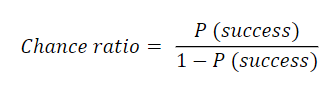
As Dias Filho and Corrar (2017) argue, the RL equation, calculates the relative probability of the occurrence of a given event or the "probability associated with each observation in odds ratio, which represents the probability of success compared to that of failure," expressed in the manner presented in the equation:
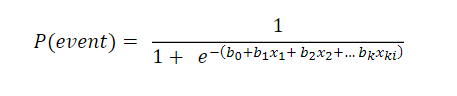
Also for Dias Filho and Corrar(2017), in a more simplified way, the logistic equation can assume the format presented in the equation:
RL uses the logistic curve to demonstrate the relationship between the independent and dependent variables using the interval between 0 and 1 (HAIR JR. et al., 2009). This probability of occurrence or prediction is based on the values of the independent variables and the estimated coefficients. It can be characterized that if the predicted probability is greater than 0.50, then it is predicted that the outcome is 1 (the event occurred); otherwise, the outcome is predicted to be 0 (the event did not occur) (Hair JR. et al., 2009). Figure 1 illustrates RL.
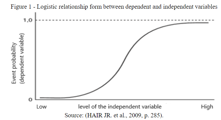
Figure 1
Logistic relationship form between dependent and independent variables
Source: (HAIR JR. et al., 2009, p. 285).
2.3 Credit scoring modeling work
Credit modeling work uses various techniques, including RL, on data prepared from companies based on information generated by financial statements. This data is taken from companies that have structured accounting information, capable of generating financial and accounting indicators.
These indicators generate information that is later treated as variables in the application of a credit scoring model. For companies that are not required to publish information, the credit scoring models use data from the customer's file, credit data, and internal history. Frame 2 presents the work developed in the modeling area, focused on credit scoring modeling.

Frame 2
Works developed in the credit scoring modeling area
Source: Study Data
It is important to note the degree of significance of the results achieved by the models presented in Frame 2, with a variation between 61.3% and 93.1% of hits on the authors' techniques (AD, RL, ANN, and their HYBRID variations). The studies that used the RL technique obtained significant results, demonstrating efficiency in the identification of variables.
It is observed that of the works listed in Frame 2, only the work of Selau and Ribeiro (2011) uses data from the registry (focused on analyzing credit for individuals), the others used, in whole or in part, information from accounting. This view reinforces the importance of the study for granting credit directed to legal entities using non-accounting information, due to the difficulty of obtaining information or the lack of it for SMEs.
3 Methodology
This research is of applied nature, which seeks the immediate solution of concrete problems of everyday life through practical guidance aimed at management and decision making (DUARTE; FURTADO, 2014). As for the research objectives, it is characterized as explanatory. According to Gil (2009), in the search to answer the "why" of things, explanatory research aims to identify factors that contribute to the occurrence of phenomena and knowledge of reality requiring sufficient and detailed description.
3.1 Methodological Procedures
For the procedures, 11 steps were applied to develop the credit scoring models, which are presented in Frame 3 and explained in the following.
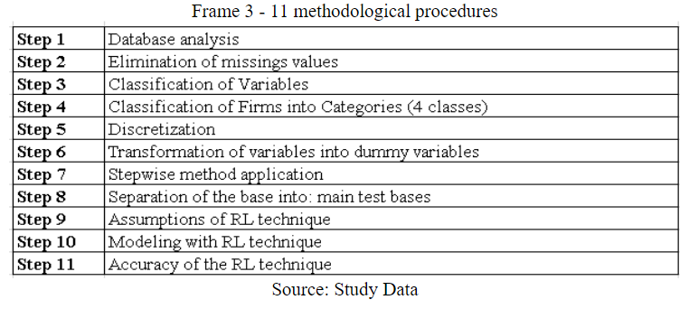
Frame 3
11 methodological procedures
Source: Study Data
Step 1: Database analysis - Observations and data were collected through reports available at the financial institution, focused on commercial and industrial lending. The name and other identifying information of the customers were replaced by random numbers to ensure anonymity.
Step 2: Elimination of missing data (missings values) - In this step, the database was analyzed, and 219 contracts were eliminated from the total of 1,710, leaving a base of 1,491 contracts. The analysis was focused on finding missing information in the independent variables for all contracts. The data collection period corresponds to active claims up to October 10, 2017. This process of eliminating missing data was also adopted by (CAMARGOS, Marcos; CAMARGOS, Mirela; ARAÚJO, 2012).
The process of "missing or lost data", for Rodrigues and Paulo (2017), corresponds to any systematic event external to the respondent, leading primarily the researcher to seek the reasons inherent to these. The justification for eliminating the data lies in the need for information to classify the size of the companies. It is noteworthy that the missing data were not captured due to being part of another system (database), not being possible to access on the date of the data survey.
Step 3: Classification of Variables - The response variable refers to the quality of credit, being identified as either performing or defaulter. According to the institution's policy, defaulters are those who are more than 30 days past due without interruption during the fiscal year. On the other hand, the clients identified with payments with no arrears or with arrears of 30 days or less were classified as defaulters.
Data Preparation: Quantitative variables can be measured on scales presented in discrete or continuous form. Qualitative variables do not have quantitative values, also known as categorical, and can be classified into nominal and ordinal (RODRIGUES; PAULO, 2017). Due to the peculiarity of the database referring to a specific cooperative and credit institution, some variables are self-explanatory, but others require clarification, they are: City Code - identifies the federation unit; Cnae - is the code that identifies the economic activity, it can also be used to facilitate the framing of the company; Value of the Guarantee - Specifies the value that the customer has in guarantee of the credit operations; Risk - Is the framing of the company with the financial institution of the probability of default; Number of Products - specifies the quantity of products that the customer has acquired from the financial institution, in force on the date of the data survey; Value of the Capital Share - Corresponds to the value, in national currency, that the customer has deposited on the occasion of the acquisition of the cooperative's shares; Size of the Companies - Identifies the classification of the company, by means of the income/invoicing presented by the company that is under analysis.
Frame 4 presents the variables that were used in the models, their orders, and codifications originated from the database provided by the Financial Institution, called primitive variables.
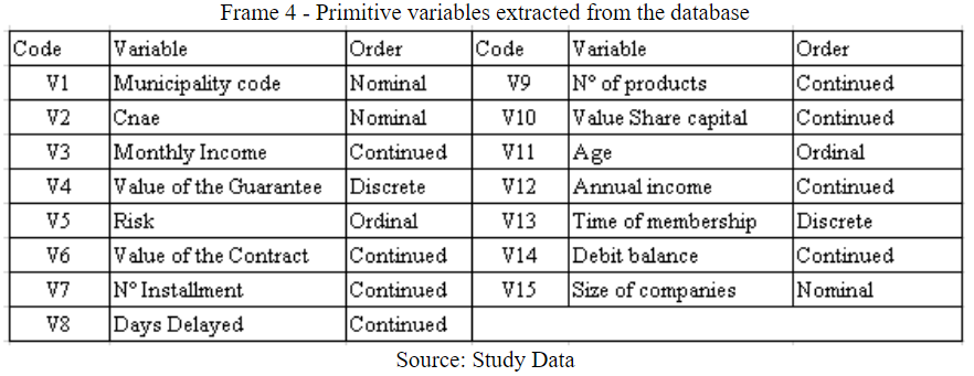
Frame 4
Primitive variables extracted from the database
Source: Study Data
Part of the variables used in this study was also found in other authors' studies as shown in Frame 05.
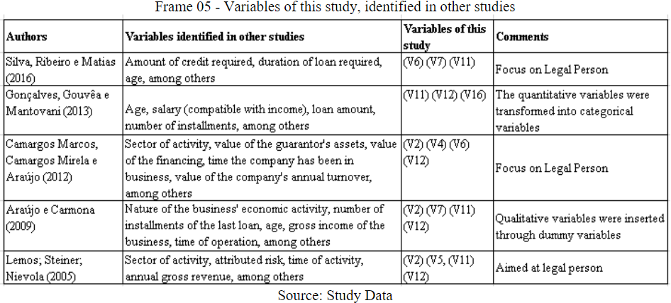
Frame 5
Variables of this study, identified in other studies
Source: Study Data
Variables (V9) and (V10) were not found in the works related to the Legal Entity in Frame 5.
Step 4: Division of company classes - The importance of recognizing the existing differences between classes of companies makes it possible to analyze them, more specifically, within their forms of performance and management. Also understanding that, when in situations of market recession, they are usually the first to present difficulties and the ones that take a longer time to recover (SILVA, 2016).
Small Companies, characterized as Micro-entrepreneur (MEI), Microenterprise (ME), Small Company (PE), differ from Medium Enterprises (MedE), as well as differ among themselves, in their structural forms, barriers, tax benefits among others, presenting different realities, generating their own information within their universe of operation. In this context, the segmentation into classes is relevant, as it makes it possible to treat the variables and their values within the reality of the companies' performance in the market.
Due to the peculiarities of the source of information, specific to each company's format, as described by Alvim (1998), as to the challenge of making available adequate information that can support the decision-making process, the proposed models were prepared as of the individual characteristics of each company category, namely: MEI, ME, PE and MedE. Companies are distributed according to BNDES (2010) ranges (or classes), in which the MEI range was included according to Law 128/2008, which changed Law 123/2006, the Microenterprise Law. The adopted classification is illustrated in Frame 6.
| Range | Up to R$60 thousand | From R$60 thousand to R$2.4 million | From R$ 2.4 million to R$16 million | From R$16 million to R$90 million |
SPSS Statistics® software was used to model credit scoring using the RL technique. Five credit scoring models were developed, one for each company class and another model for the general database described as DG.
Step 5: Discretization of variables - The variables age, annual income, length of membership, debit balance, number of installments, and contract value, were discretized. They argue, García et al. (2013), that discretization can be observed as a data reduction method, reducing a large volume of data into subsets, as it maps the data from a huge set of numerical values to a greatly reduced subset of discrete values. As a cutoff point in the calculated mean and standard deviation was (+/- 1 standard deviation) for creating the data subsets within each company category, i.e.: MEI, ME, PE, MedE, and DG. According to Lunet, Severo, and Barros (2006), the standard deviation value reflects the variability of the observations about the mean, characterized as a measure of dispersion.
Step 6: Dummy variables - After the discretization, the variables: age, annual income, membership time, debit balance, number of installments, and contract value, were transformed into dummy variables, creating a new variable for each discretized range/class, which resulted in theemergence of 23 new variables, replacing the primitive variables. According to Missio and Jacobi (2007), the dummy variable is an artificial variable that takes on a value equal to 0 or 1, indicating the absence or presence of some attribute, transforming the regression model into a flexible tool to deal with problems encountered in empirical studies. Cunha and Coelho (2017), indicate that the use of the dummy can improve the percentage of the coefficient of determination (R2) and its contribution is to indicate the presence or absence of a certain attribute, assuming only 0 or 1.
Step 7: Selection of variables - stepwise method - For the selection of variables, the stepwise method was applied. This statistical method allows determining a set of significant variables, implying the inclusion or removal of potential variables (DINIZ; LOUZADA, 2013). The stepwise method is used in estimation methods, with a sequential selection of variables, aiming to identify the independent variable with the highest predictive power in the RL model (HAIR JR. et al., 2009).
Step 8: Model validation and adjustment- For the selected techniques, a test base (BT) of 20% of the total data, chosen at random, was used for model validation. The remaining 80% of the base, called the main base (BP), was used for model fitting and elaboration. This procedure was carried outfor all 4 classes of firms and the DGs. This percentage is also found in the works of (SELAU e RIBEIRO, 2009; SILVA; RIBEIRO; MATIAS, 2016).
Step 9: Assumptions of the RL technique- In Table 1, the assumptions necessary for the development of the technique are presented.
| Logistic regression | Non linear | a. Correlation test | a. Tolerance |
| b. Absence of multicolinearity among the independent variables | b. Inverse of Tolerance (VIF) | ||
| c. Likelihood | |||
| d. Hosmer and Lemeshow |
Step 10: Model elaboration - Based on the selection of variables with greater predictive power, after using the stepwise method and the RL technique, 5 credit scoring models were elaborated, one for each class of company: MEI, ME, PE, MedE, and DG.
Step 11: Accuracy of the RL Technique - One of the ways used to verify the ability of models is through their predictive ability, also understood as accuracy. Within the RL process, the classification of the overall accuracy is generated, and then comparative analysis of the overall accuracy (prediction) of the RL technique for the 4 classes of companies versus DG is performed.
4 Results
The RL technique was applied on the contract database of a financial institution with a time cut on October 10, 2017. The database was initially separated by billing range, as illustrated in Frame 5. Also, with the information collected, the database was used to formulate a general model (DG).
4.1 Preliminary Analysis
Initially, before the approach with the test samples, a more detailed observation of the database was made in order to eliminate possible inconsistencies due to missing, obtaining a total volume of 1,448 clients, after eliminating the inconsistent data.
For the dependent variable was assigned a value of "0" for Defaulter Customers/Companies and a value of "1" for Defaulter Customers/Companies. The cutoff point used to develop the RL technique was 0.50, as highlighted in item 2.3.
4.2 Analysis of variables
When starting the database analysis, the behavior of each independent variable was observed in relation to the dependent variable and consequently among the independent variables themselves. Variables V3 (Monthly Income) and V15 (Classification) were removed from the model because they were interrelated with other variables, presenting a correlation. The existence of correlation is determined when the independent variables, among themselves, explain the same fact with similar information, this phenomenon is known as multicollinearity. For Hair Jr. et al. (2009), multicollinearity, a measure of tolerance, denotes that two or more independent variables are highly correlated when a variable can be predicted by other variables with low explanatory power for the set. In turn, variable V5 (Risk) is calculated, by the Financial Institution, based on the evolution of variable V8 (Days of Delay), both being discarded.
4.3 Discretization of variables
For a better fit of the models, observing the classes of the companies, the variables, age, annual income, membership time, outstanding balance, number of installments, and contract value, were discretized. Each of these variables, through discretization, using as parameter (+/-) 1 standard deviation, was divided into subsets, within the same variable. Subsequently, the general data group was subdivided into smaller groups of 3 to 4 subsets per variable.
4.4 Transformation of the variables into dummies
The incorporation of dummy variables to linear regression models makes them able to deal with many problems encountered in an extremely flexible way, especially in empirical studies (MISSIO; JACOBI, 2007). The variables age (V11), annual income (V12), membership time (V13), debt balance (V14), number of installments (V7), and contract value (V6) were transformed into dummy variables.
For this transformation, the subsets, already determined by the discretization, were used as a reference for the classification ranges, for each new dummy variable. Through this transformation process, 23 new dummy variables emerged to replace the primitive variables, V6, V7, V11, V12, V13, and V14, for each class of companies, separated by billing category and for the DGs.
4.5 Logistic Regression
Using a dichotomous variable as the dependent variable, the RL technique has been widely used as a prediction tool. This technique makes it possible to circumvent problems such as homogeneity of variance and normality in the distribution of errors (DIAS FILHO; CORRAR, 2017).
To structure the credit scoring models, 5 primitive variables were used, namely: (V1, V2, V4, V9 V10) and 23 dummies variables, also known as artificial variables, replacing the primitive variables (V6, V7, V11, V12, V13, and V14), totaling 28 variables, as described in Frame 7. For the interpretation of Frame 7, the following abbreviations are highlighted: P = Primitives; MV = Missing Values; PS = Substituted Primitives; PU = Used Primitives and Ar = Artificial.
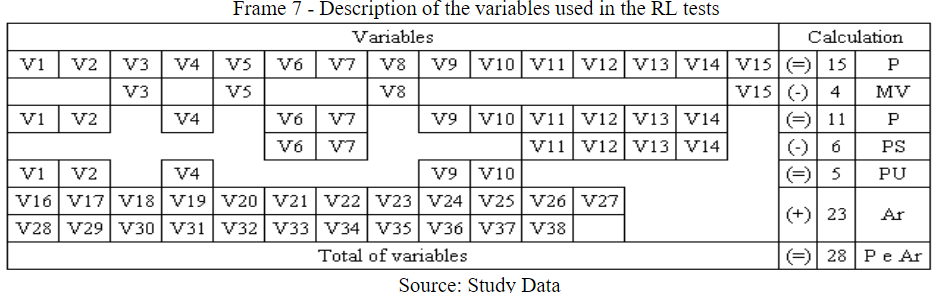
Frame 7
Description of the variables used in the RL tests
Source: Study Data
To select independent variables, which have the highest predictive power, to incorporate the prediction model for each class of companies, the stepwise method was used, according to the option made available by the SPSS® software. The cutting level adopted was 0.50 for the significance of the selection and grouping of "client" contracts, where the compliant assumed the coding value "0" and the delinquent the value "1", in the volume of the 28 independent variables used as input in the credit scoring models, after using the stepwise method.
As already mentioned, this method performs a sequential selection, aiming to identify the variable that presents a higher predictive power for the regression (HAIR JR. Et al., 2009). Na output of 9 variables with discrimination power was obtained, as shown in Table 2.
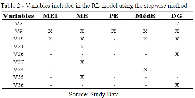
Table 2
Variables included in the RL model using the stepwise method
Source: Study Data
Table 3 presents the volume of cases that were used for the (BT) and (BP). It is observed that, within the database, the Microenterprise contains the largest volume of cases and consequently the largest volume of negotiations for the institution. Another noteworthy factor is in the number of independent variables selected by the stepwise method.
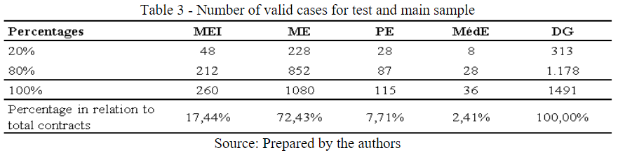
Table 3
Number of valid cases for test and main sample
Source: Prepared by the authors
4.6 Multi-collinearity test
This test consists in examining the correlation between independent variables, occurring when two or more explanatory variables try to explain the same fact (CUNHA; COELHO, 2017). Collinearity can be measured by tolerance and its inverse, called Variance Inflation Factor (VIF), being quite common measures for collinearity (HAIR JR. et al., 2009). The tolerance is calculated as 1 - R2* and the VIF is calculated using the inverse of the tolerance, when the VIF is 1 and the tolerance is 1, it implies that there is no multicollinearity (HAIR JR. et al., 2009). Table 4 presents the collinearity statistics for the 4 classes of firms and DG.
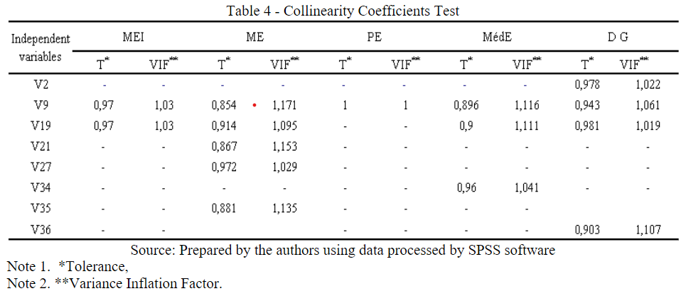
Table 4
Collinearity Coefficients Test
Source: Prepared by the authors using data processed by SPSS software
Analyzing the results, the tolerance values were very close to 1, and the VIF was also very close to 1 and far from 10. According to Hair Jr. et al. (2009), a very common cut-off reference is a tolerance value of 0.10, which corresponds to a VIF value of 10.
4.7 Likelihood Ratio Test
The Log-Likelihood Value test aims to estimate the probability of an event occurring, gauging the model's ability (DIAS FILHO; CORRAR, 2017). The test is also important to verify whether the model improves with the inclusion or removal of independent variables, as shown in Table 5. In RL, a base model is estimated, which has the function of serving as a standard for comparisons, using the sum of squares of the means to establish the value of the logarithm of the likelihood {-2LL} (HAIR JR. et al., 2009).
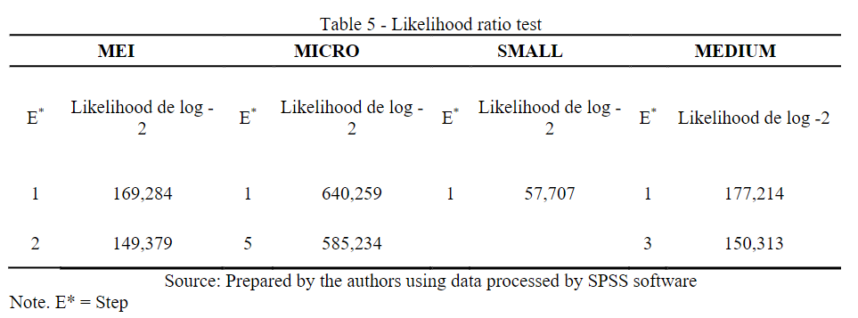
Table 5
Likelihood ratio test
Source: Prepared by the authors using data processed by SPSS software
Smaller values of measure -2LL, improve the model fit, being this technique used by the stepwise method for improvement of the previous step (stage), (HAIR JR. et al., 2009). It is observed that in all stages there was a reduction of log -2 for all steps of the company classes. Another instrument used for measuring competing models was Nagelkerke, which presented the indices: 0.388, 0.491, 0.376, and 0.427 respectively the rank order of the companies.
Table 6 presents the results for the Hosmer and Lemeshow test. According to Dias Filho and Corrar (2017), this test aims to verify whether there are significant differences between the classifications performed by the model and the observed realities. Its analysis is based on the significance of the model, which is favorable when the significance level is equal to or greater than 0.05. Of the classes presented in Table 6, the only class that did not show a significant level was Small Business, thus rejecting the null hypothesis of no significant differences. However, the stepwise method presented only one step, and there was no other level to make a comparison.
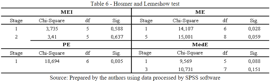
Table 6
Hosmer and Lemeshow test
Source: Prepared by the authors using data processed by SPSS software
4.8 Credit scoring models with the RL statistical technique
The variables selected to compose the credit scoring model must have the power to influence or have the possibility of influencing, a customer to either default or be in default to the extent of their influence. As Dias Filho and Corrar (2017) state, "the effect that an independent variable has on the dependent variable should be analyzed when the others remain unchanged.
As for the sign of the variables, it should be noted that a positive variation in a negative coefficient suggests a reduction in the probability of default. In case the coefficient is positive, it suggests a probability of increasing default.
Table 7 presents the weights assigned to each independent variable incorporated into the model corresponding to the class of firms selected by the stepwise method.
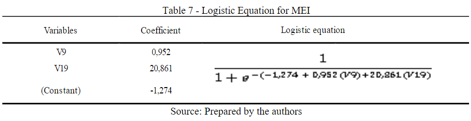
Table 7
Logistic Equation for MEI
Source: Prepared by the authors
The model, presented in Table 7, which composes the Logistic Equation for companies classified as MEI, highlights the inclusion of 2 variables, being a primitive (V9) and an artificial one (V19).
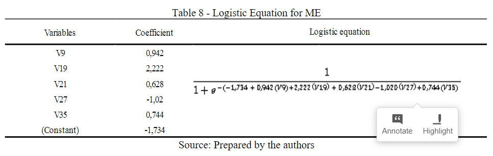
Table 8
Logistic Equation for ME
Source: Prepared by the authors
The model, presented in Table 8, which composes the Logistic Equation for companies classified as ME, highlights the inclusion of 5 variables, being one primitive (V9) and 4 dummy variables (V19), (V21), (V27), and (V35)
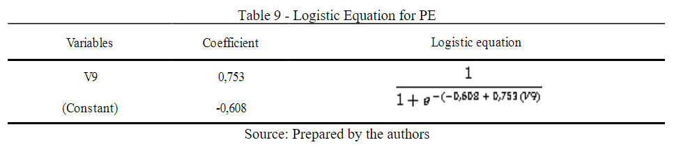
Table 9
Logistic Equation for PE
Source: Prepared by the authors
The model, presented in Table 9, which composes the Logistic Equation for companies classified as PE, highlights the inclusion of only one variable, being it primitive (V9). The selection of only one variable to compose the model is in line with the academic issue since it respects the premises of the technique but may make it difficult to accept at the management level. Improving the model with the inclusion of management or risk restriction variables may improve model reliability.
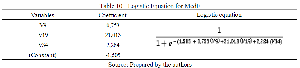
Table 10
Logistic Equation for MedE
Source: Prepared by the authors
The model, presented in Table 10, which composes the Logistic Equation for the companies classified as MedE, highlights the inclusion of 3 variables, being a primitive (V9) and 2 dummy variables (V19) and (V34)
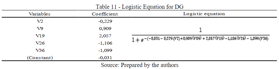
Table 11
Logistic Equation for DG
Source: Prepared by the authors
The model, presented in Table 11, which makes up the Logistic Equation for the firms classified as DG, highlights the inclusion of 5 variables, being twoprimitives (V2), (V9), and 3 dummy variables (V19), (V26) and (V36).
It can be observed that the DG model, through the stepwise method, included a maximum of 5 variables, presenting the same number of variables as the ME model, this being the class that presents the largest volume of data.
4.9 Discussion of the discriminatory power of RL
In Frame 8 through 12, the results of the BT, and BP accuracy tests for each of the firm classes and DG are presented. Frame 13 illustrates the summary of the accuracy tests, already discussed in Frame 8 through 12, along with the accuracy-test on DG, involving 1,491 cases.
By observing Frame 8, the results of the accuracy test for MEI, presented a superiority of 3.8% percentage points, of the BP over the BT, but both indicators were above 65%. The overall accuracy reached a percentage of 83.0%, in which it is interesting to note that the prediction for the defaulter reached a percentage of 93.6%, showing greater discriminatory power for identification of the defaulter. Due to the low amount of data that made up the test sample, observations for defaulters in the BT were not selected.
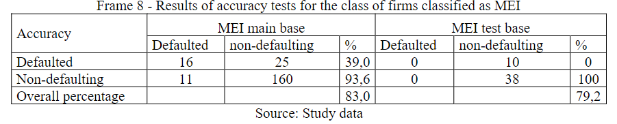
Frame 8
Results of accuracy tests for the class of firms classified as MEI
Source: Study data
In Frame 9, the accuracy for the FC class between BT and BP presents a small difference of 2.8% percentage points, this proximity demonstrates good adaptability of the model, with an overall accuracy of 84.9%. The Microenterprise, in BP, presented a predictive power for the defaulter of 64.1%, and a very significant accuracy for the defaulter of 91.1%
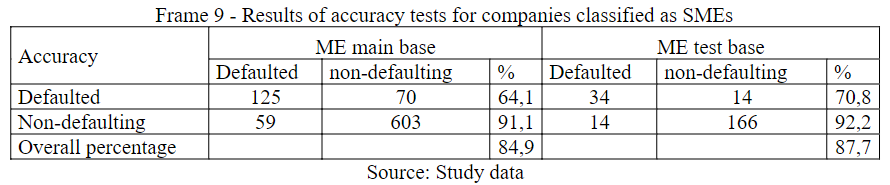
Frame 9
Results of accuracy tests for companies classified as SMEs
Source: Study data
Frame 10 illustrates the accuracy results for the companies classified in the PE class. The level of accuracy between BT and BP presented a difference of 5.2% percentage points, demonstrating the model's prediction capacity, over the BP of 88.5%, composed of 212 contracts. The percentage of correctness, about the defaulter, must be analyzed with care since it presents a percentage below 50%, this fact may be related to the volume of contracts included in the test.
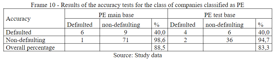
Frame 10
Results of the accuracy tests for the class of companies classified as PE
Source: Study data
Frame 11 illustrates the accuracy obtained for the MedE class. The volume of contracts used in the BP was 227 contracts, presenting an accuracy of 83.3%. The BT presented an accuracy of 100% both for defaulters and defaulters, however, the volume of contracts that composed the BT was only 12, which may distort the observed values.
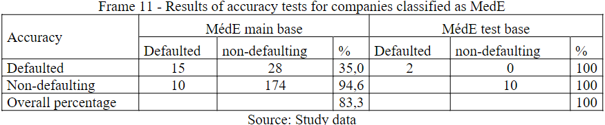
Frame 11
Results of accuracy tests for companies classified as MedE
Source: Study data
Subsequently to the application of the RL technique, in the classes: MEI, ME, PE and MedE, on the volume of contracts/clients, the general base was used, here called DG, with 1,491 valid observations, in which the same procedures of the company classes were applied.
The results are illustrated in Frame12, with LV and BP presenting almost equal accuracy, that is, 85.4% and 85.0%, respectively. The model's predictive ability was good, showing, especially, that the accuracy intended to predict the defaulter had a good performance. When analyzing the defaulter, the performance was only regular, reaching 59% and 52.5%.
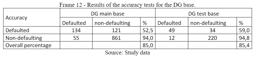
Frame 12
Results of the accuracy tests for the DG base.
Source: Study data
In the observation of Frame 13, the DG was with percentages close to the classes of companies, especially MEI and ME, however, even small percentage variations can represent significant values. An important observation is that the models with similar accuracy are those that have the largest databases, however, the PE and MEI classes are the classes that have smaller distances within the database, as can be seen in the discretizations.
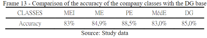
Frame 13
Comparison of the accuracy of the company classes with the DG base
Source: Study data
It can be observed that RL presents good adherence to the assumptions. For Dias Filho and Corrar (2017), the logistic model more easily accommodates categorical variables, being one of the reasons that it becomes a good alternative to Discriminant Analysis.
By analyzing Frame 13 it can be seen that the PE class of companies presents the best predictive percentage, but when observing the composition of the variables in the model for PE, according to Table 2, only one variable was selected by the stepwise method. For practical use of the model for PE, it is recommended that other variables, not covered in this study, be tested for inclusion, to make the model more robust.
In Table 3, it is also possible to observe that the ME class of companies is the one that has the most business ties in the credit portfolio with the Financial Institution, representing 72.43% of the total number of contracts. This percentage shows that the vast majority of the institution's customers have billing within the ME characteristics. Due to this factor, the accuracy of this technique becomes important for the analysis of the institution's customer portfolio, which performed in 84.9%.
It was observed that the accuracy percentages of the four classes of firms: MEI, ME, PE, and MedE, are close, but not equal to that of the DGs. Frame 14 illustrates the distribution of accuracy in increasing order, where it can be seen that the MEI, MedE, and ME classes are up to 2 percentage points below the DGs and the PE class is 3.5 percentage points above the DGs.
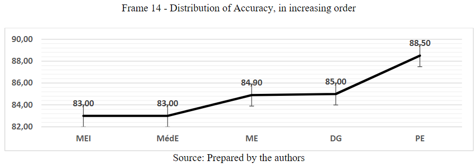
Frame 14
Distribution of Accuracy, in increasing order
Source: Prepared by the authors
These percentage differences, especially that of the FC, which represents 72.43% of the business generated by the institution, must be analyzed within each class in comparison to the risk that it presents to the financial institution.
5 Final considerations
Given the growing search for aid techniques that can generate risk indicators or measurements, this paper has developed methodological procedures, aimed at improving the information base and procedures for developing credit scoring models, using the RL technique on the database of a Financial Institution.
Due to the peculiarities of the sectors, size, and know-how, among other factors, that may be related to risk, we sought to develop credit scoring models for each class of company. The general base data, provided by the financial institution, are specific to clients classified as small and medium-sized companies. Silva (2016) reinforces that smaller companies are more sensitive and that in times of market financial constraints, they are the first to face financial difficulties and consequently the last to emerge from these difficulties.
Given the above, a methodology was formulated with 11 steps, seeking to show the path taken and the improvements incorporated into the process, such as discretization, creation of artificial variables, division of the database into four classes of companies according to their market performance reality. With the improvement in the methodological procedures, it was possible to increase the volume of variables in the models, with influence on possible changes in customer status. These procedures contributed to the elaboration of five credit scoring models, one for each class and one more model for DG.
It was possible to observe that, although some variables are common to all classes and DG, other independent variables were incorporated only in one or another model. This observation becomes important since it allows verifying that for a certain class of companies, such variable must be analyzed in a specific way, justifying the elaboration of the model by class of companies. In particular, variables V9 and V10, incorporated into the study, were not identified in the articles researched for the development of this work.
The methodological procedures contributed to improving model accuracy by incorporating and analyzing each variable added to the model and its influence after discretization and the creation of "dummies" artificial variables. As for the RL accuracy percentages, good results were obtained for the company and DG classes, demonstrating that, despite the existence of other techniques that emerged later, such as computational or genetic algorithms, RL is still a technique with good applicability.
The accuracy values achieved, in general, for the technique tested, were higher than 65%, and the results obtained are in line with those observed in recent research by Selau and Ribeiro (2011), Prado et al. (2016), Louzada, Ara and Fernandes (2016), and Mselmi, Lahiani and Hamza (2017). It is noteworthy that the variables used in the models are not derived from accounting, financial or economic indicators, but rather from sources of registration and credit history and customers, for example, billing, membership time, number of products, age, among others.
The models presented, using the RL technique, can serve as a basis for institutions that work with financial development and that have in their portfolio companies classified as, for example, SMEs. However, it should be noted that the statistical test that shows how much the variation is explained by the models is not yet satisfactory, and the inclusion of other variables can improve the robustness of the models. On the other hand, regarding the model for ME and PE, there was a very reduced selection of explanatory variables, limiting its use as a decision support tool.
Finally, we can highlight the peculiarities of the models proposed for legal entities, such as division of the base in company classes respecting their differences and the use of non-accounting or auditable variables in their entirety.
Future studies could consider the use of other methods, such as computational, genetic algorithms, or hybrid systems, in the search for indicators with greater predictive power for the four classes of companies, as well as the study to include other variables in the composition of the models.
REFERENCES
ALVIM, P. C. R. C. O papel da informação no processo de capacitação tecnológica das micro e pequenas empresas. Ciência da Informação, Brasília, v.27, n.1, p. 28-35, 1998.
ARAÚJO, E. A.; CARMONA, C. U. M. Construção de modelos credit scoring com Análise Discriminante e Regressão Logística para a gestão do risco de inadimplência de uma instituição de microcrédito. Revista Eletrônica de Administração, v.15, n.1, 2009.
BANCO NACIONAL DE DESENVOLVIMENTO - BNDES. Classificação de porte de empresa.Disponível em: . Acesso em: 11 nov 2017.
BERGER, N. A.; COWAN, A. M.; FRAME, W. S. The surprising use of credit scoring in small business lending by community banks and the attendant effects on credit availability, risk, and profitability. Journal of Financial Services Research, v.39, n.1, p. 1–17, 2011.
BERTI, A. Consultoria e Diagnóstico Empresarial. 2.ed. Curitiba: Juruá, 2012.
BRASIL, Lei nº 128, de 19 de dezembro de 2008,Presidência da República. Casa Civil.Subchefia para Assuntos Jurídicosteoria e prática. Disponível: . A cesso em: 12 ago 2017.
BRASIL, Lei nº 123, de 14 de dezembro de 2006,Presidência da República. Casa Civil.Subchefia para Assuntos Jurídicosteoria e prática. Disponível:http://www.planalto.gov.br/ccivil_03/Leis/LCP/Lcp123.htm. Acesso em: 12 ago 2017.
BRUNI, A. L. A análise contábil e financeira. 4. ed. São Paulo: Atlas. 2010.
CAMARGOS, M. A. DE.; CAMARGOS, M. C. S.; ARAÚJO, E. A. A inadimplência em um programa de crédito de uma instituição financeira pública de minas gerais: uma análise utilizando Regressão Logística, REGE, São Paulo, v.19, n.3, p. 467–486, 2012.
CIAMPI, F.; GORDINI, N. Small Enterprise Default Prediction Modeling through Artificial Neural Networks: An Empirical Analysis of Italian Small Enterprises. Journal of Small Business Management, v.51 n.1, p.23-45, 2013.
CUNHA, J. V. A.; COELHO, A. C. Regressão Linear Múltipla. In: Corrar, L. J. (Coord.); Paulo, E. (Coord.); Dias F ilho, J. M. (Coord.). Análise Multivariada: para os Cursos de Administração, Ciências Contábeis e Economia. São Paulo: Atlas, cap. 3, 2017.
DIAS FILHO, J. M.; CORRAR, L. J. Regressão Logística. In: Corrar, L. J. (Coord.); Paulo, E. (Coord.); Dias F ilho, J. M. (Coord.). Análise Multivariada: Para os Cursos de Administração, Ciências Contábeis e Economia. São Paulo: Atlas, cap. 5, 2017.
DINIZ, C.; LOUZADA, F. Métodos Estatísticos para Análise de Dados de Crédito. In: 6th BRAZILIAN CONFERENCE ON STATISTICAL MODELLING IN INSURANCE AND FINANCE. Maresias – São Paulo, ABE, USP, UNICAMP 24 a 28 de março 2013.
DUARTE, S. V.; FURTADO, M. S. V. Trabalho de conclusão de curso em Ciências Sociais Aplicadas. 1.ed. São Paulo: Saraiva, 2014.
GARCÍA S. et al. A survey of discretization techniques: Taxonomy and empirical analysis in supervised learning. IEEE Transactions on Knowledge and Data Engineering, v.25 n.4, p.734-750, 2013.
GIL, A. C. Métodos e Técnicas de Pesquisa Social, 7.ed. São Paulo: Atlas, 2009.
GONÇALVES, E. B.; GOUVÊA, M. A.; MANTOVANI, D. M. N. Análise de risco de crédito com o uso de Regressão Logística. Revista Contemporânea de Contabilidade. UFSC, Florianópolis, v.10, n.20, p.139-160, 2013
GOUVÊA, M. A.; GONÇALVES, E. B. Análise de risco de crédito com o uso de modelos de Regressão Logística e redes neurais. Globalização e Internacionalização de Empresas, X SEMINÁRIO EM ADMINISTRAÇÃO FEA-USP, 09 a 19 de agosto 2007.
HAIR JR, et al.Análise multivariada de dado. Tradução Adonai Schlup Sant’Anna. 6.ed. Porto Alegre: Bookman, 2009.
KELLY, M. G.; HAND, D. J. Credit scoring with uncertain class definitions.IMA Journal of Management Mathematics, v. 10, n. 4, p. 331-345, 1999.
LEMOS, E. P.; STEINER, M. T. A.; NIEVOLA, J. C. Análise de crédito bancário por meio de redes neurais e árvores de decisão: uma aplicação simples de data mining. Revista deAdministração. São Paulo, v.40, n.3, p.225-234, jun./ago./set, 2005.
LI, K.; NISKANEN, J.; KOLEHMAINEN, M. Financial innovation credit default hibrid model for SME lending. Expert Systems With Applications, v.61 p. 343-355, 2016.
LOUZADA, F.; ARA, A. FERNANDES, G. B. Classification methods applied to credit scoring: Systematic review and overall comparison. Surveys in Operations Research and Management Science. v.21 n.2, p.117– 134, 2016.
LUNET, N.; SEVERO, M.; BARROS, H. Desvio padrão ou erro padrão: Notas Metodológicas. ArquiMed, 2006. Disponível: http://www.scielo.mec.pt/pdf/am/v20n1-2/v20n1-2a08.pdf. Acesso em: 15 jan. 2018.
LUO, C.; WU, Desheng.; WU, Dexiang. A deep learning approach for credit scoring using credit default swaps. Engineering Applications of Artificial Intelligence, v.65, p 465-470, October 2017.
LUO, S.; KONG, X.; NIE, T. Spline based survival model for credit risk modeling. European Journal of Operational Research, v.253. n.3, p 869-879, September 2016.
MARQUÉS, A. I.; GARCÍA, V.; SÁNCHEZ, J. S. Exploring the behaviour of base classifiers in credit scoring ensembles. Expert Systems with Applications, v.39 n.11, p.10244–10250, September 2012.
MARQUES, J. M.; LIMA. J. D. de. A estatística multivariada na análise econômico-financeira de empresas. Revista FAE, Curitiba, v.5, n.3, p.51-59, 2002.
MILERIS, R. Macroeconomic Determinants of Loan Portfolio Credit Risk in Banks. Inzinerine Ekonomika-Engineering Economics,v.23 n.5, p.496–504, 2012.
MISSIO, F.; JACOBI, L. Variáveis dummy: especificações de modelos com parâmetros variáveis. Ciência e Natura, v.29, n.1, p.111-135. 2007.
MSELMI, N.; LAHIANI, A.; HAMZA, T. Financial distress prediction: The case of French small and medium-sized firms. International Review of Financial Analysis. v.50 p. 67-80, 2017.
OHLSON, J. A. Financial Ratios and the Probabilistic Prediction of Bankruptcy. Journal of Accounting Research, v.18 n.1, p.109-131, 1980.
PRADO et al. Multivariate analysis of credit risk and bankruptcy research data: a bibliometric study involving different knowledge fields (1968–2014). UFLA. Scientometrics. v.106, n.3, p. 1007–1029, 2016.
RODRIGUES, A.; PAULO, E. Introdução à Análise Multivariada. In: Corrar, L. J. (Coord.); Paulo, E. (Coord.); Dias F ilho, J. M. (Coord.). Análise Multivariada: para Curso de Administração, Ciências Contábeis e Economia. São Paulo: Atlas, cap. 1, 2017.
ROGERS, Dany.; MENDES-DA-SILVA.W.; Rogers Pablo. Credit Rating Change and Capital Structure in Latin America. Brazilian Administration Review - BAR, v.13, n2, p.1–22, 2016.
SELAU, L. P. R.; RIBEIRO, J. L. D. Uma sistemática para construção e escolha de modelos de previsão de risco de crédito. Gestão e Produção, v.16, n.3, p.398-413, 2009.
SELAU, L. P. R.; RIBEIRO, J. L. D. A systematic approach to construct credit risk forecast models. Pesquisa Operacional, v.31 n.1, p. 41–56, 2011.
SILVA, R. A.; RIBEIRO, E. M.; MATIAS, A. B. Aprendizagem estatística aplicada à previsão de default de crédito. Revista de Finanças Aplicadas, v.7, n.2, p.1-19, 2016.
SILVA, J. P. D. Análise Financeira das Empresas. São Paulo: Atlas, 2004.
SILVA, J. P. D. Gestão e Análise de Risco de Crédito. 9.ed. rev. e atualizada. São Paulo: Cangage Learning, 2016.
SMARANDA, C. Scoring Functions and Bankruptcy Prediction Models: Case Study for Romanian Companies. Procedia Economics and Finance, v.10, p.217-226, 2014.
VENTURA, R. Mudanças no Perfil do Consumo no Brasil; Principais Tendências nos Próximos 20 Anos. Macroplan – Prospectiva, Estratégia e Gestão, agosto2010.
ZHU, Y.et al. Predicting China’s SME credit risk in supply chain financing by logistic regression, artificial neural network and hybrid models. Sustainability (Switzerland), v.8, n.5, p.1-17, 2016.