Artículos
High grade glioma segmentation in magnetic resonance imaging
Segmentación de glioma de alto grado en imágenes de resonancia magnética
 Miguel Vera
Yoleidy Huérfano
Luis Javier Martínez
Yudith Contreras
Williams Salazar
María Isabel Vera
Oscar Valbuena
Maryury Borrero
Carlos Hernández
Doris Barrera
Ángel Valentín Molina
Juan Salazar
Elkin Gelvez
Frank Sáenz
Diego Hoyos
Yeny Aria
Miguel Vera
Yoleidy Huérfano
Luis Javier Martínez
Yudith Contreras
Williams Salazar
María Isabel Vera
Oscar Valbuena
Maryury Borrero
Carlos Hernández
Doris Barrera
Ángel Valentín Molina
Juan Salazar
Elkin Gelvez
Frank Sáenz
Diego Hoyos
Yeny Aria
High grade glioma segmentation in magnetic resonance imaging
Revista Latinoamericana de Hipertensión, vol. 13, no. 4, pp. 323-329, 2018
Sociedad Latinoamericana de Hipertensión
Resumen: A través de este trabajo se propone una técnica computacional para la segmentación de un tumor cerebral, identificado como un glioma de alto grado (HGG) de tipo astrocitoma anaplásico de grado III, que está presente en las imágenes de resonancia magnética (MRI). Esta técnica consta de 3 etapas desarrolladas en el dominio tridimensional. Ellas son: preprocesamiento, segmentación y postprocesamiento. La etapa de preprocesamiento utiliza una técnica de umbralización, un filtro de erosión morfológica (MEF), en escala de grises, seguido de un filtro de mediana y de un algoritmo de magnitud de gradiente. Por otro lado, con el propósito de generar una segmentación preliminar del HGG, durante la etapa de segmentación se implementa un algoritmo de agrupamiento, llamado crecimiento de regiones (RG), que se aplica a las imágenes preprocesadas. El RG requiere para su inicialización la ubicación de un vóxel semilla cuyas coordenadas se obtienen, automáticamente, a través del entrenamiento y la validación de un operador inteligente basado en máquinas de vectores de soporte (SVM). Debido a la alta sensibilidad del RG a la ubicación de la semilla, la SVM se implementa como un clasificador binario altamente selectivo. Durante la etapa de post-procesamiento, se aplica un filtro de dilatación morfológica a la segmentación preliminar, generada por RG. El error relativo porcentual (PrE) se considera para comparar las segmentaciones de la HGG generadas de forma manual por un neurooncólogo, con las segmentaciones dilatadas de la HGG, obtenidas automáticamente. La combinación de parámetros vinculados al PrE más bajo permite establecer los parámetros óptimos de cada uno de los algoritmos computacionales que componen la técnica computacional propuesta. Los resultados obtenidos permiten reportar un PrE de 11.10%, lo cual indica una buena correlación entre las segmentaciones manuales y las producidas por la técnica computacional desarrollada.
Palabras clave: Imágenes cerebrales por resonancia magnética, Tumor cerebral, Gliomas de alto grado, Astrocitoma anaplásico de grado III, Técnica computacional, Segmentación.
Abstract: Through this work we propose a computational technique for the segmentation of magnetic resonance images (MRI) of a brain tumor, identified as high grade glioma (HGG), specifically grade III anaplastic astrocytoma. This technique consists of 3 stages developed in the three-dimensional domain. They are: pre-processing, segmentation and post-processing. The pre-processing stage uses a thresholding technique, morphological erosion filter (MEF), in gray scale, followed by a median filter and a gradient magnitude algorithm. On the other hand, in order to obtain a HGG preliminary segmentation, during the segmentation stage a clustering algorithm called region growing (RG) is implemented and it is applied to the pre-processed images. The RG requires, for its initialization, a seed voxel whose coordinates are obtained, automatically, through the training and validation of an intelligent operator based on support vector machines (SVM). Due to the high sensitivity of the RG to the location of the seed, the SVM is implemented as a highly selective binary classifier. During the post-processing stage, a morphological dilation filter is applied to preliminary segmentation generated by RG. The percent relative error (PrE) is considered by comparing the segmentations of the HGG, generated manually by a neuro-oncologist, with the dilated segmentations of the HGG, obtained automatically. The combination of parameters linked to the lowest PrE, allows establishing the optimal parameters of each computational algorithms that make up the proposed computational technique. The obtained results allow reporting a PrE of 11.10%, which indicates a good correlation between the manual segmentations and those produced by the computational technique developed.
Keywords: Magnetic resonance brain imaging, Cerebral tumor, High grade glioma, Grade III anaplastic astrocytoma, Computational technique, Segmentation.
INTRODUCTION
The segmentation of anatomical structures of the human brain, present in images acquired by any imaging modality, constitutes the starting point for the diagnosis of a large number of diseases or pathologies that affect the brain. Among these pathologies are brain tumors which originate from several cell lines and are classified according to several criteria1. One of these is according to the place of the body where they are generated. In this sense, they can be classified into two groups: a) Primary tumors. Space-occupying lesions composed of cells (SOLC) that start in the brain and tend to remain there. b) Secondary tumors, SOLC that originate in other sites of the human body and spread and/or infiltrate, such as metastasis, in the brain the most frequent metastases come from cancers that usually occur in human skin, lungs and breast2,3.
The World Health Organization (WHO) uses the degree of malignancy of the tumor as a criterion to classify primary tumors into four grades. According to this classification, tumors labeled with grades I and II are generally benign; while those classified in grades III and IV are considered malignant. Normally, patients with primary grade I brain tumors have a longer survival than those with grade IV tumors1,2,3.
Gliomas are primary tumors arising from glial cells and they can also be classified by grade according to WHO grading system.. It classifies gliomas with histopathological criteria and the grade of gliomas is highly correlated with prognosis5.
Furthermore, gliomas can be classified into high-grade gliomas (HGG) and low-grade gliomas (LGG). Anaplastic astrocytomas and glioblastoma multiform tumors are included in HGG; while grade II astrocytoma (Astrocite) and oligoastrocytomas, are included in LGG6. For the present study, the tumors reported in the literature as HGG are of special interest. Additionally, an anaplastic astrocytoma is a grade III tumor, type HGG, that infiltrates diffusely in the neoplasm that confirms a focal or scattered anaplasia. Its histological diagnosis is based on nuclear atypia and mitotic activity. Anaplasic astrocytomas appear more frequently in younger adults. Approximately 4% of people with anaplastic astrocytomas have several tumors at the time of diagnosis.7.
According to WHO4., the HGG grade III anaplasic astrocytoma can be located in the context illustrated in figure 1.
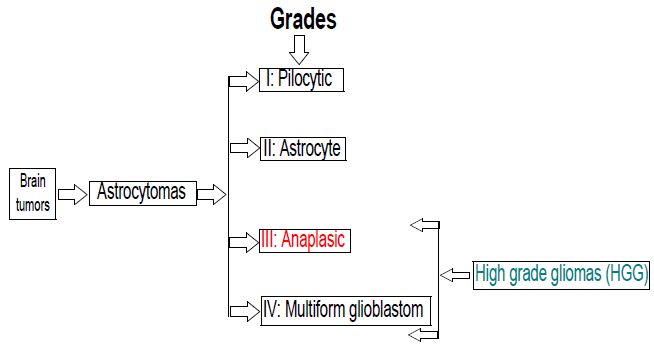
Figure 1.
Block diagram with a classification linked to the brain tumor considered in the present work.
It is known that cerebral digital neuroimages are accompanied by various imperfections such as noise8,9,10 and artifacts8 which affect the quality of information associated with the anatomical structures that make up these images. These imperfections become real challenges, when computational strategies are implemented to generate the morphology (normal or abnormal) of the mentioned structures8. By way of example, figure 2, generated based on magnetic resonance images (MRI), illustrates the presence of Rician noise, the stair artifact, the low contrast between brain structures and the meningioma (structure with red cross in its center).
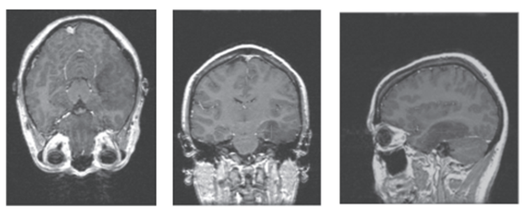
Figure 2.
Perpendicular views of brain MRI in which it is possible to observe Rician noise, low contrast between lobular structures and the anaplasic astrocytoma (Red cross).
Additionally, when reviewing the state of the art regarding tumor segmentation, the works described below were found. In this sense, Jones et al.11, present a novel whole-brain diffusion tensor imaging (DTI) segmentation (D-SEG) to delineate tumor volumes of interest (VOIs) for subsequent classification of tumor type, MRI modality. DTI scans were obtained from 95 patients with low- and high-grade glioma, metastases, and meningioma and from 29 healthy subjects. D-SEG uses .-means clustering of the 2D space to generate segments with different isotropic and anisotropic diffusion characteristics. Classification of tumor type using D-SEG was performed using support vector machines (SVM). The results point at the SVM classified tumor type with an overall accuracy of 94.7%, providing better classification than previously reported.
Furthermore, Cho et al.12, development a HGG and LGG classification system based on multi-modal image radiomics features. Take into account a ground true, the results point at this method covering an area under the curve of 0.8870 and achieving 0.8981, 0.8889 and 0.9074 of accuracy, sensitivity and specificity, respectively.
Alternatively, a computational technique (CT) is proposed for the segmentation of a HGG, present in a database formed by three-dimensional brain images of MSCT. This technique considers the stages of pre-processing, segmentation and post-processing Also, percent relative error (PrE). will be used to compare segmentations of the HGG obtained automatically and manually.
MATERIALS AND METHODS
Description of the databases
The database (DB) used was provided by the Central Hospital of San Cristóbal-Táchira-Venezuela. It was acquired through the MRI modality and consists of three-dimensional images (3D), corresponding to the anatomical structures present in the head of 1 male patient. Numerical characteristics are presented on table 1.
| DB Label | Voxels number | Voxels dimensions (mm3) | Age (years) |
| DB1 | 256x256x124 | 0.9375 x 0.9375x 1.5 | 47 |
In a complementary manner, manual segmentation is available, generated by a neuro-oncologist, corresponding to the HGG present in the DB considered. This segmentation represents the ground truth that will serve as a reference to validate the results.
Description of the proposed computational technique, for the automatic segmentation of the HGG.
Figure 3 presents a schematic diagram that synthesizes the methods that make up the proposed technique, to segment the tumor.
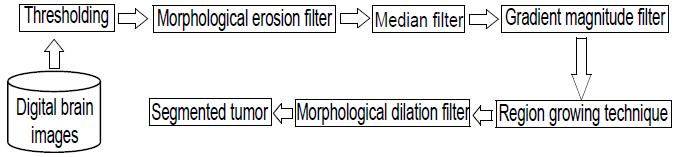
Figure 3.
Block diagram of the CT proposed for the segmentation of the HGG.
Pre-processing Stage
In the block diagram, presented in figure 3, this stage corresponds to the techniques: Thresholding, Erosion, Median and Gradient magnitude filter. Each of them is described below.
- Thresholding:
The thresholding algorithms are, generally, simple structures and allow to classify, efficiently, the elements of an image considering one or several thresholds. Such thresholds can be selected by considering both the histogram of an image and the position, intensity or an arbitrary neighborhood of the element under study, often called the current element13. In the present work a simple threshold was considered, which is based on the choice of a value for a certain threshold.
This threshold allows discrimination between the anatomical structure of interest and the rest of the structures present in an image. Usually, the referred threshold is chosen considering the histogram of the image. One of the criteria applied to perform the aforementioned discrimination is the following: If the intensity or gray level of the current element is equal to or less than the selected threshold value, the gray level (GL) of the current element remains unchanged; while if such intensity is greater than GL of the current element, it is generally correlated with the lower level of gray present in the image being processed13.
- Morphological Erosion Filter (MEF):
Mathematical morphology is based on set theory, this means the objects present in an image can be treated as sets of points. Generally, it is possible to define operations between two sets consisting of elements belonging to the objects in question and a set called structuring element (SE). SEs can be visualized as neighborhoods of the element under study, which have morphology (shape) and variable size14.
Mathematical morphology is implemented, in practice, through various morphological filters whose basic operators are erosion and dilation15,16. These operators are non-linear spatial filters that can be applied to binary, grayscale or color images.
In particular, the erosion (⊖) of a two-dimensional image (I), composed of gray levels, using a two-dimensional SE, is defined by Equation 117. 
where: min the minimum gray level contained in SE, (s, t) defines the size of the SE and (x, y) represents the position of the pixel under study.
According to equation 1, to apply the filter or morphological erosion operator the image considered with an SE or neighborhood, of arbitrary size, is covered, replacing the gray level of each of the elements of such image by the level of gray minimum, contained in the aforementioned neighborhood. For purposes of the present work, a cubic structuring element was considered and the size of said SE is left as a parameter to control the performance of the MEF.
- Median Filter (MF):
The median filter (MF) is also non-linear and normally, it is used to minimize the impulsive type noise present in the gray levels of the voxels neighboring the voxel object of study18. This type of filter is characterized by the conservation of the edges of the objects present in the image and it has the advantage that the final value of the voxel is a real value present in the image and not an average. In addition, the median filter is less sensitive to extreme values. One of the main drawbacks is that the computation time increases, substantially, as the size of the neighborhood increases19.
- Gradient Magnitude Filter (GMF):
The role of this filter is to detect the edges of the structures present in the images (I). The magnitude of the gradient is often used in image analysis, mainly to identify the contours of objects and the separation of homogeneous regions20. Edge detection is the identification of significant discontinuities in the level of gray or color images21. This technique calculates the magnitude of the gradient using the first directional partial derivatives of an image. The classic 3D mathematical model, to obtain a filtered image by magnitude of the gradient (IGM), is presented by equation 2.
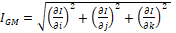 [Equation 2]
where: i, j, k represents the spatial directions in which the gradient is calculated.
In practice, the magnitude of the gradient of the image in each position of the voxel, object of study, is calculated using an approach based on finite differences. In the present work, central finite differences are used. Theoretically, the filter of magnitude of the gradient based on the intensity values is very susceptible to noise21, therefore, it is recommended to filter the image initially to improve the performance of the detector with respect to noise.
- Binary Morphological Dilation Filter (MDF):
In order to compensate the effect produced by the morphological erosion filter, the application of a morphological dilation filter (MDF) is considered, taking into account the binary image obtained by RG. The effect of morphological dilation is to enlarge the regions of the maximum intensity image. In particular, the dilation (⊕) of a two-dimensional binary image (Ib), using a bidimensional structuring element (B), is defined as the result of operating the Ib with the values of the SE under the logical operation OR14. For the purposes of this work, a cubic structuring element was considered and the size of said SE is left as a parameter to control the performance of the dilatation process.
Segmentation Stage
· Computer intelligence operators: Support Vector Machines (SVM).
Support vector machines (SVM) are paradigms that undergo training and detection processes, and are based on both the Vapnik-Chervonenkis learning theory and the minimization principle that considers structural risk. SVM can be considered as classification and functional approach tools22,23.
A variant of the SVM, called the least squares vector support machine (LSSVM), can be obtained using robust statistics, Fisher discriminant analysis and replacing the system of inequations that govern the SVM, by an equivalent system of linear equations, which can be solved more efficiently24. Additionally, unlike other learning-based classification systems such as artificial neural networks (NN), LSSVMs use the criterion of minimization of structural risk, which raises the generalization capacity of the aforementioned machines to optimum levels, making it possible for LSSVM perform adequately in the validation process, in this feature surpassing NN, which uses empirical risk24,25.
In this work, the location of the seed voxel, to initialize the segmentation technique called region growth (RG)8, is calculated using LSSVM. There are several functions that can be considered to construct the decision surface that allow the vector support machines to identify the seed. For purposes of the present work, a Gaussian radial base function (RBF) is considered and, therefore, a formulation is obtained that depends on the hyperparameters, identified as: a) Parameter for the error penalty (γ). b) To control the selectivity (σ2) of the LSSVM.
In this sense, the LSSVMs deserve a process of tuning of such hyperparameters. Theoretically, both parameters can assume values belonging to the range of real numbers comprised in 0 and infinity24. This tuning process is necessary because it is very difficult to know, a priori, the combination of values that will generate optimal results when the LSSVM carry out the training and validation processes.
Additionally, to automatically identify the coordinates of the seed voxel, the following procedure was implemented:
i) A size reduction technique, based on bicubic interpolation, optimal reduction factor, is applied to match the one obtained in6. This allows generating sub-sampled images of 64x64 pixels from filtered images of 512x512, that is, the mentioned factor is 8.
ii) A neurosurgeon selects, on the sub-sampled image, a reference point (P1) given by the centroid of the layer containing the maximum blood pool occupied by the HGG. For this point, the manual coordinates that unambiguously establish their spatial location in each considered image are identified.
iii) An LSSVM is implemented to recognize and detect point P1. For this, the processes of:
a) Training. Training circle circular neighborhoods of 10 pixels, manually traced by a neurosurgeon, containing both point P1 (markers) and regions not containing P1 (no markers) are selected as a training set. For the markers, the center of their respective neighborhoods coincides with the manual coordinates of P1, previously established.
Such neighborhoods are constructed on the axial view of a sub-sampled image of 64x64 pixels. The main reason why a single image is chosen, for each reference point, that the aim is to generate a LSSVM with a high degree of selectivity, which detects only those pixels that have a high degree of correlation with the training pattern.
Then each neighborhood is vectorized and, considering its gray levels, the attributes mean, variance, standard deviation and median, are calculated. Thus, both markers and non-markers are described by vectors (Va) of statistical attributes, given by: Va = [mean, variance, standard deviation and median].
Additionally, the LSSVM is trained considering the vectors Va as a training pattern and intoning the values of the parameters that control its performance, γ and σ.. This approach, based on attributes, allows the LSSVM to do its work with greater efficiency, than when using the larger vector-based approach, which only considers the gray level of the elements of an image.
The training set is constructed with a ratio of 1:10, which means that 10 non-markers are included for each marker. The tag +1 is assigned to the class made up of the markers; while the -1 tag is assigned to the class of non-markers, that is, the training work is done based on a binary LSSVM.
During training, a classifier with a decision boundary is generated to detect LSSVM entry patterns as markers or non-markers. Subsequently, due to the presence of false positives and negatives, a process is applied that allows incorporating into the training set the patterns that the LSSVM initially classifies inappropriately.
In this sense, it was considered a toolbox called LS-SVMLAB and the Matlab15 application to implement an LSSVM classifier based on a radial base Gaussian kernel with parameters σ2 and γ.
b) Detection. The trained LSSVMs are used to detect P1, in images not used during training. To do this, a trained LSSVM looks for this reference point, in the axial view, from the first to the last image that makes up each of the 7 databases considered.
The validation process carried out with LSSVM allows the automatic identification of the coordinates for P1 which are multiplied by a factor of 8 units, in order to be able to locate them, in the images of original size. In this way, the aforementioned coordinates are used to establish the exact location of the seed voxel required by the RG for its initialization.
Finally, as a synthesis, figure 4 illustrates the process followed to locate the seed voxel in the databases considered.
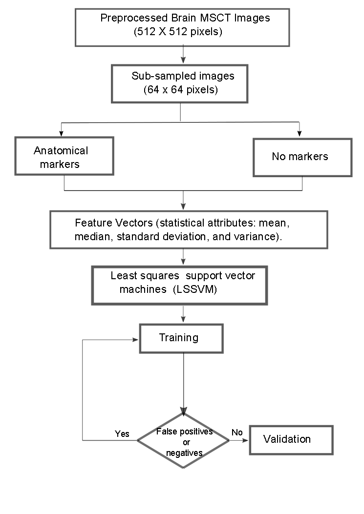
Figure 4.
Synthetic diagram that illustrates the operability of the LSSVM for the detection of the seed voxel coordinates.
· Region growing (RG).
The region growing is an unsupervised clustering technique, which performs an iterative process that attempts to characterize each of the classes, according to the similarity between the voxels that integrate each of them and thus perform the segmentation8. The RG method allows grouping the pixels or voxels belonging to the objects that make up an image according to a predefined criterion. The RG requires a "seed" point which can be selected, manually or automatically, to extract all the pixels connected to seed8.
To apply the RG, to the pre-processed images, the following considerations were made: a) The initial neighborhood, which is constructed from the seed, is assigned a cubic shape whose side depends on an arbitrary scalar r. The r parameter requires a tuning process. b) As a pre-defined criterion, modeling is chosen through Equation 4.
|I(x) − µ| < mσ (4)
Where: I(x) is the intensity of the seed voxel, μ and σ the arithmetic mean and the standard deviation of the gray levels of the initial neighborhood and m a parameter that requires tuning.
· Tuning process: Obtaining optimal parameters
The adequate performance of the proposed technique requires obtaining optimal parameters for each of the algorithms that comprise it. To do this, using DB1 as a reference, modify the parameters associated with the technique you wish to intone by systematically going through the values belonging to certain ranges, as described below.
o Erosion, Median and Dilation filters have the size of the observation window as a parameter. In order to reduce the number of possible combinations, an isotropic approach was considered to establish the range of values, which control the size of the aforementioned window, which is given by the odd combinations, given by the following ordered lists: (1,1,1), (3,3,3), (5,5,5), (7,7,7) and (9,9,9).
o The parameters of the LSSVM, σ2 and γ, are toned assuming that the cost function is convex and developing tests based on the following steps:
Ø For tuning of parameter γ, the value of σ2 is arbitrarily set and values are systematically assigned to the parameter γ. The value of σ2 is initially set at 2.5. Now, γ is varied considering the range [0,100] and a step size of 0.25
Ø An analogous process is applied to intone the parameter σ2, that is, it is assigned to γ the optimal value obtained in the previous step and, a step size of 0.25 is considered to assign to σ the range of values contained in the interval [0.50].
· The optimal parameters of the LSSVM are those values of γ and σ2 that correspond to the relative minimum percentage error, calculated considering the manual coordinates of the reference seed, established by the neurosurgeon and the automatic ones generated by the LSSVM.
o During the RG parameters tuning process, each one of the automatic segmentations of the HGG corresponding to the DB1 described, is compared with the manual segmentations of the HGG generated by a neurosurgeon, considering the PrE. The optimal values for the parameters of the RG (r and m), are matched to that experiment that generates the lowest value for the PrE.
RESULTS
Quantitative results
The optimal sizes for the Erosion, Median and Dilation filters were (3,3,3), (3,3,3) and (3,3,3), respectively. Regarding the trained LSSVM, values of 2.00 and 1.50 were obtained as optimal parameters for γ and σ2, respectively. The way to obtain these parameters is by means of the error that is presented when comparing the manual and automatic coordinates considering the percentage relative error (PrE). For this minimum value the PrE, the optimal values of RG’s parameters, r and m, were 1 and 1.7, respectively.
The best automatic segmentation of the HGG yielded a volume of 27.72 cm3; while the volume associated with manual segmentation, of the tumor, was 24.95 cm3. This imply that the minimum PrE was 11.10%.
Qualitative results
Figure 5, shows a 2-D view of both the original HGG and the processed versions after applying the proposed technique; while figure 6 shows an excellent three-dimensional representation of the segmented tumor.
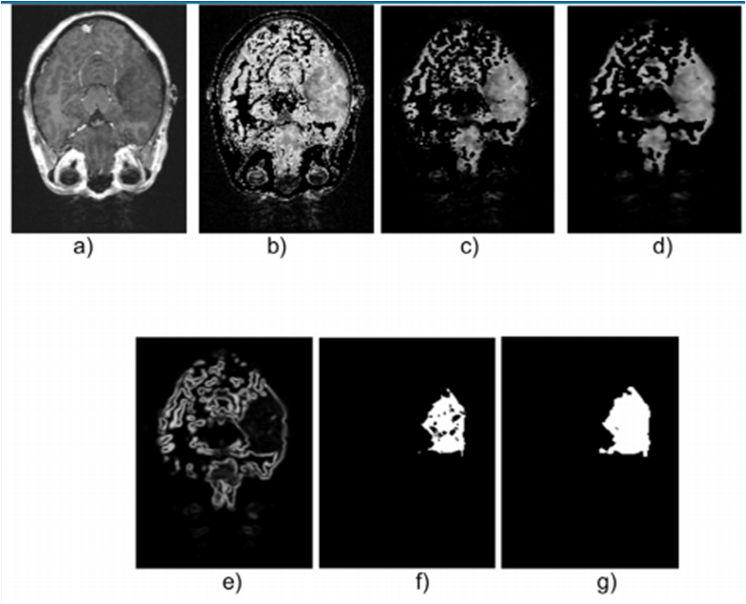
Figure 5.
Axial view of images belonging to DB1: a) Original, b) Thresholdized, c) Erode, d) Smoothed with median filter, e) Borders with gradient magnitude, f) Segmented with region growing technique, g) HGG Dilated.
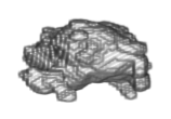
Figure 6.
3-D representation of the segmented tumor corresponding to DB1.
This figure presents the typical structure that characterizes this type of tumor. The low PrE value, obtained using the volume of the segmented HGG, shows a high precision of the developed computational technique.
CONCLUSIONS
A computational technique has been presented and its tuning process allows an accurate segmentation of HGG grade III anaplastic astrocytoma, presents in magnetic resonance images. This statement is based on the fact that the PrE obtained was very low.
The use of intelligent operators, represented by the least squares vector support machines, allowed the automatic identification of the coordinates corresponding to the seed voxel which plays a crucial role in the adequate initialization of the unsupervised grouping algorithm based on region growing.
The HGG volume is vital when deciding whether a patient is surgically treated or not, to address the tumor that affects their health status. Obviously, both the size of a HGG and its location can seriously compromise the health of a patient.
Computational techniques such as that developed in the present investigation are precise and useful to generate the exact location and precise quantification of the volume occupied by the aforementioned tumor. Additionally, the HGG segmentation is useful to plan surgery and to remove as much of the tumor as possible; while avoiding parts of the brain that control vital functions.
In the future, it is planned to carry out an inter-subject validation of the developed computational technique considering a significant number of three-dimensional images, linked to patients with this type of disease.
ACKNOWLEDGEMENTS
The authors are grateful for the financial support given by the Universidad Simón Bolívar-Colombia through the 2016-16 code project.
REFERENCES
1. Stelzer K. Epidemiology and prognosis of brain metastases. Surg Neurol Int. 2013;4(Suppl 4):S192-202.
2. Mcneill K. Epidemiology of Brain Tumors. Neurol Clin. 2016;34(4):981-998.
3. American Brain Tumor Association (ABTA). About Brain Tumors: A Primer for Patients and Caregivers. 9ª Edition. 2015 ABTA.
4. WHO (2007). Cavenee W, Louis D, Ohgaki H et al. Eds. WHO Classification of Tumours of the Central Nervous System. WHO Regional Office Europe.
5. Wu W., Lamborn K., Buckner J., Novotny P., Chang S., O’Fallon J., Jaeckle K., Prados M. Joint NCCTG and NABTC prognostic factors analysis for high-grade recurrent glioma. Neuro-oncology, 2010;12(2):164-172.
6. Bjoern H. Menze et al. The multimodal brain tumor image segmentation benchmark (BRATS). IEEE transactions on medical imaging, 2015; 34(10):1993-2024.
7. Ostrom QT, Gittleman H, Fulop J, Liu M, Blanda R, Kromer C, et al. CBTRUS Statistical Report: Primary Brain and Central Nervous System Tumors Diagnosed in the United States in 2008-2012. Neuro Oncol 2015 Oct;17 Suppl 4:iv1-iv62 PubMed ID 26511214.
8. Vera M. Segmentación de estructuras cardiacas en imágenes de tomografía computarizada multi-corte. Ph.D Thesis, Universidad de los Andes, Mérida-Venezuela, 2014.
9. Gudbjartsson H. y Patz S.The rician distribution of noisy MRI data, Magn. Reson. Med. 1995;34 (1):910-914.
10. Macovski A. Noise in MRI, Magn. Reson. Med. 1996:36 (1) 494-497.
11. Jones T., Bymes T., Yang G. Brain tumor classification using the diffusion tensor image segmentation (D-SEG) technique. Neuro-Oncology. 2015;17(3):466–476.
12. Cho H., Park H. (2017). Classification of low-grade and high-grade glioma using multi-modal image radiomics features. 39th Annual International Conference of the IEEE Engineering in Medicine and Biology Society (EMBC). 3081 – 3084.
13. Sezgin M., Sankur B. Survey over image thresholding techniques and quantitative performance evaluation. Journal of Electronic Imaging, 2004; 13(1):146–165.
14. Serra J. Image Analysis Using Mathematical Morphology. London, England: Academic Press, 1982.
15. González R., Woods R. Digital Image Processing. USA: Prentice Hall, 2001.
16. Mukhopadhyay S., Chanda B. A multiscale morphological approach to local contrast enhancement. Signal Processing. 2000; 80(4): 685–696.
17. Yu Z., Wei G., Zhen C., Jing T., Ling L. Medical images edge detection based on mathematical morphology. In Proceedings of the IEEE Engineering in Medicine and Biology 27th Annual Conference, Shanghai–China, September 2005; 6492–6495.
18. W. Pratt. Digital Image Processing. USA: John Wiley & Sons Inc, 2007.
19. Fischer M., Paredes J., Arce G. Weighted median image sharpeners for the world wide web. IEEE Transactions on Image Processing. 2002;11(7):717-27.
20. V. Vapnik, Statistical Learning Theory. New York: John Wiley & Sons, 1998.
21. E. Osuna, R. Freund, y F. Girosi. Training support vector machines: an application to face detection. In Conference on Computer Vision and Pattern Recognition (CVPR ’97), San Juan, Puerto Rico, 1997, 130–136.
22. A. Smola. Learning with kernels. Ph.D Thesis, Technische Universitt Berlin,Germany, 1998.
23. B. Scholkopf y A. Smola, Learning with Kernels: Support Vector Machines, Regularization,Optimization, and Beyond. Cambridge, MA , USA: The MIT Press, 2002.
24. J. Suykens, T. V. Gestel, y J. D. Brabanter, Least Squares Support Vector Machines.UK: World Scientific Publishing Co., 2002.
25. M. Oren, C. Papageorgiou, P. Sinha, E. Osuna, y T. Poggio. Pedestrian detection using wavelet templates. In CVPR ’97: Conference on Computer Vision and Pattern Recognition (CVPR ’97). Washington, DC, USA: IEEE Computer Society, 1997,193–200.