Carátula del artículo
Read this paper if you want to learn logistic regression
Leia este artigo se você quiser aprender regressão logística
 Antônio Alves Tôrres Fernandes antonio.alvestorres@ufpe.br
Federal University of Pernambuco, Brazil
Dalson Britto Figueiredo dalson.figueiredofo@ufpe.br
Federal University of Pernambuco, Brazil
Enivaldo Carvalho da Rocha enivaldocrocha@gmail.com
Federal University of Pernambuco, Brazil
Willber da Silva Nascimento nascimentowillber@gmail.com
Federal University of Pernambuco, Brazil
Revista de Sociologia e Política, vol. 28, no. 74, 2020
Universidade Federal do Paraná
Received: 19 October May 2019
Accepted: 07 May 2020
The least squares linear model (OSL) is one of the most used tools in Political Science (
Kruger & Lewis-Beck, 2008). As long as its assumptions are respected, the estimated coefficients from a random sample give the best linear unbiased estimator of the population’s parameters (
Kennedy, 2005). Unbiased because it does not systematically over or underestimates the parameter’s value and because it gives the smallest variance among all possible estimates (
Lewis-Beck, 1980).
What about when assumptions are violated? In that case, we must adopt techniques better suited to the nature of the data. For instance, imagine a study that investigates the impact of campaign spending on the chance of a candidate being elected or not. Since the dependent variable is binary, some assumptions of the least squares model are violated (homoscedasticity, linearity, and normality) and the estimates may be inconsistent. A logistic regression is the best tool to handle dichotomous dependent variables, that is, when
y can only take on two categories: elected or not-elected; adopted the policy or did not adopt the policy; voted for president Bolsonaro or not.
Lottes, DeMaris, and Adler (1996) argue that, despite logistic regression’s popularity in the Social Sciences, there is still a lot of confusion regarding its correct use. Given our pedagogical experience, this difficulty is explained by the lack of intuitive teaching materials. Moreover, many undergraduate and graduate programs, as well as textbooks, end their content at linear regression, shortening the dissemination of other data analysis techniques.
To fill this gap, this paper presents an introduction to logistic regression. Our goal is to facilitate the understanding of its practical application. As far as audience, we write to students in the early stages of training and teachers who need materials for quantitative methods courses. Methodologically, we reproduce data from
Castro and Nunes (2014) regarding the relationship between involvement in corruption scandals (
Mensalão2 and
Sanguessugas3 scandals) and the reelection chances for candidates running for federal deputy in Brazil in 2006. All data and scripts are available at
Open Science Framework (OSF)
4 website.
By the end, the reader should be able to identify when a logistic regression should be used, computationally implement the model, and interpret the results. We are aware that this paper does not replace a detailed reading of primary sources on the subject and more technical materials. Nevertheless, we hope to make understanding logistic regression easier to you and to disseminate replicability as data analysis teaching tool.
The remainder of the paper is divided as follows: the next section explains the underlying features logistic regression. The third identifies the main technical conditions that must be met to ensure that the model’s estimates are consistent. The fourth section describes the main statistics that must be observed. Lastly, we provide some recommendations on how to improve the quality of methodological training offered to Political Science undergraduate and graduate students in Brazil.
II. The logic of logistic regression
5
The use of binary categorical dependent variables is common in Political Science empirical research. For example: voted or not (Nicolau, 2007;
Soares, 2000), won or lost the electoral contest (
Speck & Mancuso, 2013;
Peixoto, 2009), adhered to the policy or not (
Furlong, 1998), democracy or not-democracy (
Goldsmith, Chalup & Quinlan, 2008), started a war or not (
Henderson & Singer, 2000), appealed a judicial ruling or not (
Epstein, Landes & Posner, 2013). For all these situations, a logistic regression is the best suited technique to model the dependent variable’s variation given a set of independent variables.
In a logistic regression, the dependent variable only has two categories
6. Generally, the occurrence of the event is coded as 1 and its absence as 0. Keeping in mind that codification changes the coefficients’ signal and, therefore, their substantive interpretation. To better understand how a logistic regression works, it is necessary to understand the logic of regression analysis as a whole. Let’s look at the linear model’s classic notation:
(1)
Y represents the dependent variable, that is, what we are trying to understand/explain/predict. X represents the independent variable. The intercept, (α), represents the value of Y when X equals zero. The regression coefficient, (β), represents the variation observed in Y associated with the increase of one unit of X. The stochastic term, (ε), represents the error of the model. Technically, it is possible to estimate if there is a linear relationship between a dependent variable (Y) and different independent variables. Moreover, the model allows the observation of the effect magnitude and to test the coefficients’ statistical significance (p-value and confidence intervals).
A logistic regression can be interpreted as a particular case of generalized linear models (GLM)
7, in which the dependent variable is dichotomous. Figure1 compares the linear and logistic models.
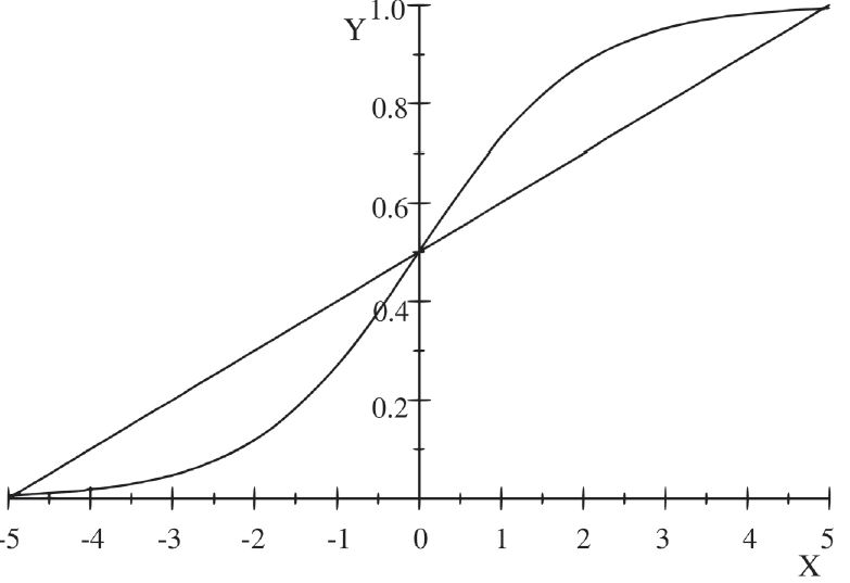 Figure 1
Linear regression line versus logistic curve
Figure 1
Linear regression line versus logistic curve
Source: The authors, based on Hair, A.
et al. (2019).
Because the dependent variable in the logistic model takes on only two values (0 or 1), the probability predicted by the model must also be limited to that interval. When X (independent variable) takes on lower values, the probability approaches zero. Conversely, as X increases, the probability approaches 1. For
Kleibaum and Klein (2010), that logistic functions vary between 0 and 1 explains the model’s popularity. Given that the dependent variable’s binary nature violates some the linear model’s assumptions (homoscedasticity
8, linearity
9, normality), using a linear model to analyze binary variables may generate inefficient and biased coefficients
10. To better understand the relationship between linear and logistic models, we reproduced the data from
Hosmer, Lemeshow, and Sturdivant (2013) on the association between age and coronary disease (Graph 1)
11.
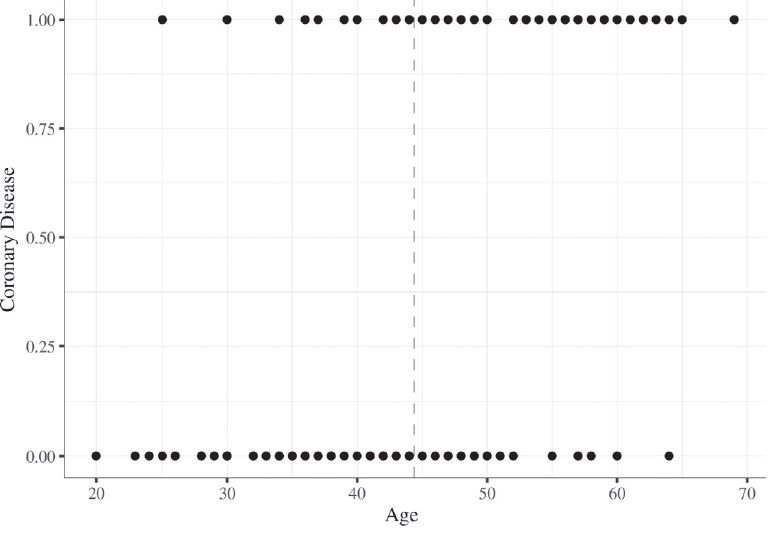 Graph 1
Age x coronary disease
Graph 1
Age x coronary disease
Source: The authors based on and
Hosmer, Lemeshow, and Sturdivant (2013).
The vertical dashed line represents the age mean: 44,38 years old. The cases were coded as 1 (developed coronary disease) and 0 (did not develop it). The trend is very clear: as age increases, the amount of people diagnosed with coronary disease grows. An intuitive way to observe this pattern is to examine the number of cases using the mean as a parameter for comparison. For example, for people above the mean there more illness cases, while for people below the mean, the larger concentration is in the “did not develop it” category. That is, the graph is stating that there is an association between age and coronary disease. It is in that sense that a logistic regression informs the probability of the event coded as 1 occurring, in the case at hand, developing coronary disease.
Table 1 presents the data by age group.
Table 1
Age group x coronary disease
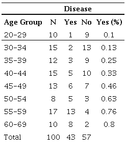
Simply observe the last column to reach the same conclusion presented by Graph 1: the higher the age, the higher the chance to develop coronary diseases. An additional option to visualize the relationship between these variables is to graphically represent the percentage of people who are ill for each age group (Graph 2).
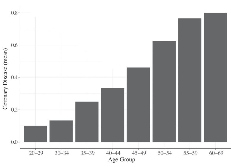 Graph 2
Age group x coronary disease
Graph 2
Age group x coronary disease
Source: The authors based on
Hosmer, Lemeshow, and Sturdivant (2013).
We observe a positive correlation between age (axis X) and the probability to develop cardiac diseases (axis Y) is observed. A logistic regression will inform the direction, magnitude, and the statistical significance level of this relationship. In a nutshell, the researcher must use a logistic regression when the dependent variable is categorical and binary. Given that many variables in the Humanities are categorical, the analytical benefits associated with the correct application and interpretation of a logistic regression are evident
12.
III. Planning a logistic regression
Table 2 describes the five stages that should be observed.
Table 2
Planning a logistic regression in five stages
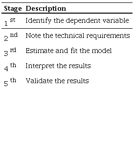
The first stage is to identify a research question for which the dependent variable is naturally dichotomous. For example, given the popularity of logistic regression in health research, commonly used variables are: lived/died; sick/not sick; smoker/ non-smoker. Usually, a researcher must forgo from recoding a continuous or discrete variable into a dichotomous categorical one. More clearly, let’s say the interest variable is income per capita. It is wrong to recode income to produce two categories: rich versus poor. Technically, recoding a quantitative variable into a categorical one implies loss of information and that reduces the estimates’ consistency (
Fernandes
et al., 2019
)
13.
At the second stage, the technical requirements must be observed. Despite being more flexible than other statistical techniques, logistic regression is sensitive to, for example, problems of multicollinearity (high levels of correlation between independent variables)
14. There are different procedures to minimize this problem. The simplest is to increase the number of observations (
Kennedy, 2005). An additional option is to use some data reduction technique to create a synthetic measure from the variance of the original variables. We must not simply exclude one of the independent variables, under the risk of producing errors in the model specification. In a logistic regression, the size of the sample is key (Hair
et al., 2009). Small samples tend to produce inconsistent estimates. On the other hand, excessively large samples increase the power of statistical tests in such a way that any effect tends to be statistically significant, regardless of magnitude.
Hosmer and Lemeshow (2000) suggest a minimal
n of 400 cases.
Hair
et al. (2009)
suggest a ratio of 10 cases for each independent variable included in the model.
Pedhazur (1982) recommends a ratio of 30 cases for each estimated parameter.
Another eventual source for problems is outliers. Extreme cases produce disastrous results in data analysis and in the case of a logistic regression, the presence of atypical observations may harm the model’s fit. Once aberrant cases are detected, a researcher must decide what to do with them. Sometimes an extreme case is nothing more than a typo and can be easily solved. One option is to exclude outliers from the model’s estimation and measure the impact of its inclusion on the coefficients. Another procedure commonly adopted is to recode the case, giving it a less extreme value, the mean for example. In any case, it is important to describe in detail what was done to deal with eventual extreme observations
15.
At stage three, the researcher must estimate the model. Here, two procedures are essential: a) report the software and b) and share replication materials, which include the original data, the manipulated data, and the computational scripts
16. These procedures increase transparency and make replicability of results easier (
King, 1995;
Paranhos
et al., 2013
;
Janz, 2016;
Figueiredo Filho
et al., 2019
). After estimating the model, the next step is evaluating the goodness of the fit. This can be done by comparing the null model (just the intercept) with the model that incorporates the independent variables. A statistically significant difference between the models indicates that the explanatory variables help to predict the occurrence of the dependent variable.
Figure 2 shows the underlying logic of model comparison when we are using logistic regression.
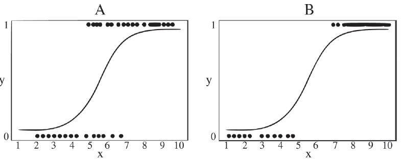 Figure 2
Comparing the fit of logistic models
Figure 2
Comparing the fit of logistic models
Source:
Hair
et al. (2009)
.
Comparatively, model B has a better fit than model A. This can be observed given the difference in discriminatory power. While model A presents high variability, model B is more precise. For Tabachnick, Fidell, and Ullman,
[...] “logistic regression, like multiway frequency analysis, can be used to fit and compare models. The simplest (and worst-fitting) model includes only the constant and none of the predictors. The most complex (and ‘best’-fitting) model includes the constant, all predictors, and, perhaps, interactions among predictors. Often, however, not all predictors (and interactions) are related to the outcome. The researcher uses goodness-of-fit tests to choose the model that does the best job of prediction with the fewest predictors.” (
Tabachnick, Fidell & Ullman, 2007, p. 439).
The fourth stage is the interpretation of results. Unfortunately, many works limit themselves to analyzing the statistical significance of the estimates and do not pay attention to the coefficients’ magnitude. We suggest that researchers interpret the coefficients and substantively discuss how results are related to the research hypothesis. Unlike a linear regression, in which coefficients are easy to interpret, the estimates produced in the logistic model are less intuitive
17. This is because the logit transformation informs the independent variable’s effect on the variation of the dependent variable’s natural logarithm of the odds. For example, when considering a coefficient of 0.6, an increase of 0.6 units is expected in the logit of Y every time X increases by one unit. This approach’s main disadvantage is its lack of intelligibility. To state that the amount in logit in
18 creased 0.6 units is not very intuitive and does not help to understand the relationship between the variables.
A second possibility is to analyze the independent variables’ impact on the odds of Y. To do so, a researcher must get the exponent of the coefficient itself. In our example, the exponential of 0.6 is 1.82. This means that for each additional unit in X, an increase of 1.82 is expected in the chance of Y occurring, keeping other variables constant. Graph 3 illustrates the distribution of a simulation’s exponential function, in which x varies between -5 and 5.
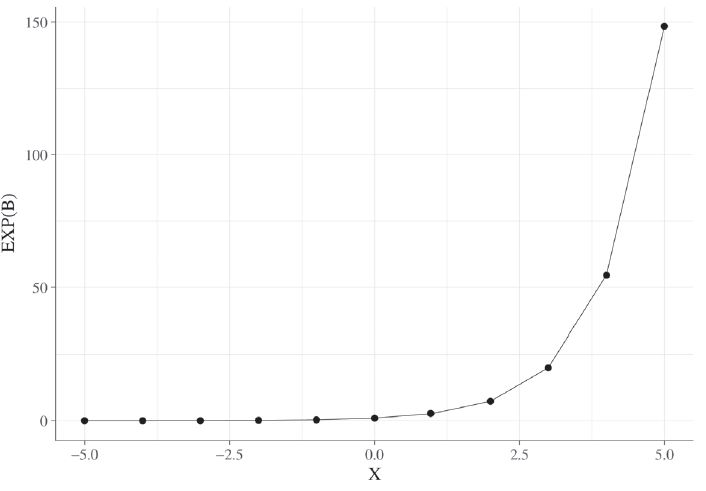 Graph 3
Exponential function
Graph 3
Exponential function
Source: The authors, based on
Hosmer, Lemeshow, and Sturdivant (2013).
In a logistic regression, the exponential of a positive value (+) produces a coefficient larger than 1. Conversely, a negative coefficient (-) returns a Exp (β) smaller than 1. A coefficient with a value of zero produces an Exp (β) equal to 1, indicating that the independent variable does not affect the chance of the dependent variable’s occurrence. So, write it down in your notebook: the farther the coefficient is from one, regardless of the direction, the greater the impact of a given independent variable on the chance of the event of interest occurring
19.
The third possibility is to estimate the percentage increase in the chance of the occurrence of Y. To do so, one must subtract one unit from the exponentiated regression coefficient and multiply the result by 100, in this case (1.82-1 * 100). Then we have that the increase in one unit of X is associated with an increase of 82% in the chance of Y occurring (
ceteris paribus). The interpretation of the logistic regression’s coefficients may become a little more complicated when the chance is smaller than 1, that is, when the coefficient (β) is negative. One solution is to invert the coefficient (1/coefficient’s value), which makes the interpretation easier. For example, a coefficient of 0.639, when inverted, indicates that when the independent variable decreases by in one unit, an average increase of 1.56 is expected in the chance of the dependent variable occurring.
Lastly, the researcher must validate the results observed with a subsample of its original dataset. This procedure gives the research results more reliability, especially when working with small samples. According to
Hair
et al. (2009)
,
“the most common approach for establishing external validity is the assessment of hit ratios through either a separate sample (holdout sample) or utilizing a procedure that repeatedly processes the estimation sample. External validity is supported when the hit ratio of the selected approach exceeds the comparison standards that represent the predictive accuracy expected by chance.” (Hair
et al., 2014, p. 329).
Unfortunately, this procedure is rarely used by political scientists. We suspect that the reduced use of validation is in part explained by the lack of training on the specificities of logistic regression. The next section presents an applied example of logistic regression and explains how the results should be interpreted.
IV. An applied example
To illustrate the application of the logistic regression, we replicated the data from
Castro and Nunes (2014) on corruption and reelection
20. However, since our focus is purely methodological, we will not explore the substantive meaning of the conclusions reported by the authors. According to the planning from the previous section, the first step is to identify the dependent variable that will take value “1” for candidates reelected in 2006 and “0” if otherwise
21.
The second step is to verify the technical requirements to estimate the logistic regression. During this step, it is important to observe the presence of outliers, the occurrence of high correlation between independent variables, and an adequate sample size. Due to space limitations, we will reproduce only one of the models presented by
Castro and Nunes (2014). Specifically, the sample used to estimate model 5 from
Table 6 (p. 41), which has a total of 217 observations and a proportion of 19 cases for each independent variable. We do not find deviant cases and the level of correlation between the variables included in the model is acceptable. Thus, we can move on to the next phase.
The third stage consists of the model’s estimation:
22
(2)
Chart 1 summarizes how the variables were measured.
Chart 1
Variables measurement level
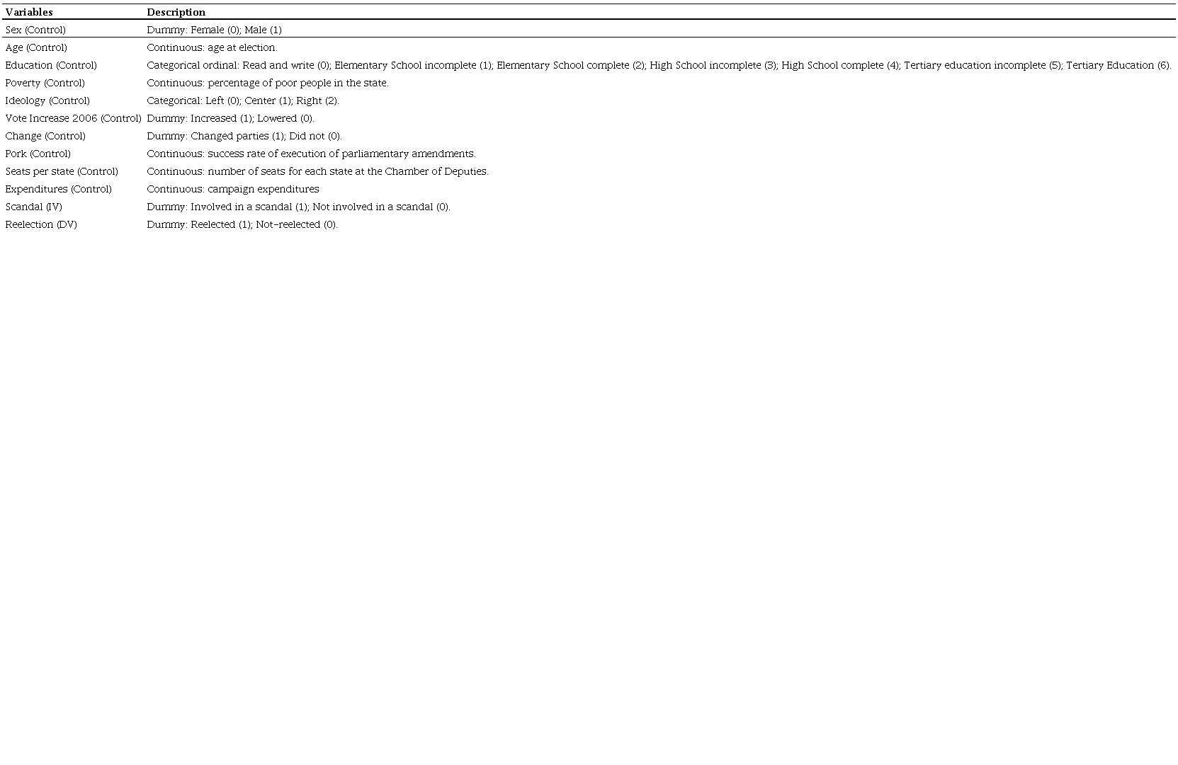
We will test three hypotheses:
H1: being involved in a corruption scandal reduces the probability of reelection;
H2: the higher campaign spending, the higher the probability of reelection;
H3: the higher the execution of amendments, the higher the probability of reelection.
V. Results
The first step is to analyze the distribution of the dependent variable.
Table 3 summarizes this information.
Table 3
Frequency distribution for the independent variable (reelected)
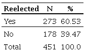
There is information for 451 cases. From this total, 60.53% of the federal deputies were reelected in 2006, which means 273 occurrences
23. We can say then that the probability for reelection is of 0.605. Alternatively, the chance of being reelected can be calculated by the division between the probabilities (yes/no), here, 0.605/0.395 = 1.53.
Table 4 illustrates this information.
Table 4
Comparison of reelection rate (involved x not-involved) (%)
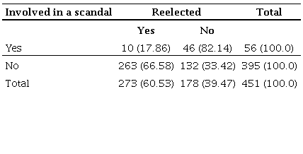
Considering only candidates involved in corruption scandals, the reelection rate was 17.86%, since 10 out of 56 representatives got a new term
24. This means that, for this group, the probability for reelection is 0.179 and the chance for reelection is 0.22. For the candidates not involved in corruption scandals, the chance of being reelected is 1.9. Ultimately, in our replication example, the logistic regression consists of the comparative analysis of the reelection percentage of candidates involved in corruption scandals and those not involved
25.
In terms of the model’s general fit, one of the main tests used is the
Hosmer and Lemeshow (2000). This test is considered more robust than a common chi-square, especially when there are continuous independent variables or when the sample’s size is small (
Garson, 2011).
Table 5 summarizes the information of interest (value of the test, degrees of freedom, and statistical significance) for Hosmer and Lemeshow tests, and
Table 6 shows the same for the Omnibus test of model coefficients.
Table 5
Hosmer and Lemeshow Test

Table 6
Omnibus test of model coefficients
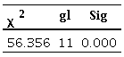
A non-significant result (p > 0.05) suggests that the model estimated with the independent variables is better than the null model. The estimated model has a chi-square (χ
2) of 6.832 and a p-valor of 0.555, suggesting an adequate fit. Another commonly used adjustment measure is the Omnibus test of model coefficients. It is a chi-square test comparing the model’s variance with the independent variables and the null model (just the intercept).
Unlike the Hosmer and Lemeshow test, a significant result (p < 0.05) suggests an adequate fit. According to the data, the model has a chi-square of 56.356 (p-value < 0.001), that is, the fitted model is better than the null model. The, we should conclude that the independent variables influence the dependent variable’s variation
26. We do not find these tests in Castro and Nunes’s paper (2014), nor the computational scripts.
Table 7 summarizes the coefficients estimated by the logistic regression model in an attempt to reproduce the results reported in
Table 6 of
Castro and Nunes (2014).
Table 7
Logistic regression model coefficients
*
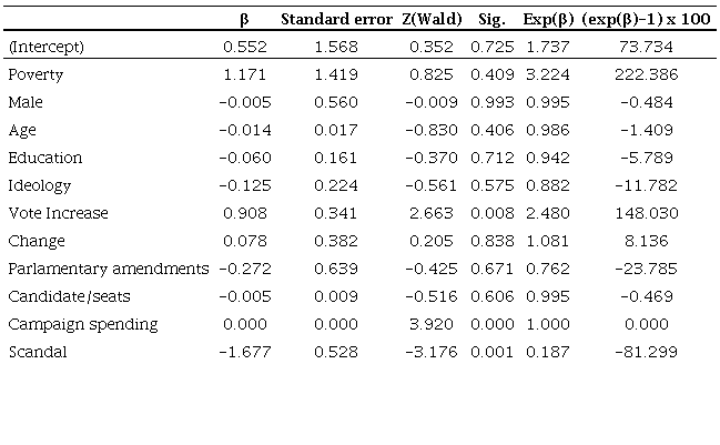
As with a linear regression, the first step is to analyze the estimated coefficients (β). Here, the research must observe the sign of the estimates and compare them with the direction expected in their hypotheses. X
11 (Scandal) has a negative effect (-1.677) on the probability of reelection. Unlike a linear model, logistic regression coefficients does not have an direct interpretation.
There are two main ways of reading the coefficients: a) analyze the odds ratio and b) turn the odds ratio into a percentage. With the former, we conclude that involvement in corruption scandals reduces the chances of being elected. In terms of percentages, being involved in corruption diminishes in 81.2% the probability of being reelected, as theoretically expected by hypothesis 1. When considering campaign expenses, the effect was null, with an Exp (β) = 1.000.
As in
Castro and Nunes (2014), we did not find significant effects of the parliamentary amendment variable on the chance of reelection, considering the magnitude of the p-value and the standard error twice as large as the estimate of the impact itself
27.
After analyzing the coefficients associated with the variables of interest, the next step is to evaluate the quality of the model’s fit.
Table 8 summarizes some goodness-of-fit measures typically reported in models estimated by the maximum likelihood
28.
Table 8
Model goodness-of-fit measures
*
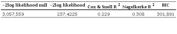
It is common for statistical packages to show in the output the number of iterations used by the computer to estimate the model. Informing that the model converged after iteration 5 means that the coefficients were estimated via maximum likelihood. Generally, the faster a model converges (less iterations), the better. If the model does not converge, the coefficients are unreliable. One of the main factors that explain a model’s non-convergence is the insufficiency of cases in relation the number of independent variables included in the model.
According to
Menard (2002), the log likelihood is a measure of parameter selection in the logistic regression model. However, most statistical packages report the -2 log likelihood (-2LL) and its interpretation is as follows: the larger it is, the worse is the model’s explanatory/predictive capacity. Intuitively, it can be interpreted as a measure of the error when trying to use a determined set of independent variables (model) to explain the dependent variable’s variation. The researcher can request the iteration history of the estimation. The procedure will produce the -2 log likelihood of the null and the fitted models. The difference between them is measured with a chi-square. As it is an error measure, the larger the chi-square, the larger is the error reduction of the fitted model (with the independent variables), in relation to the null model.
Table 8 presents the value of -2LL to make comparing the models easier. In the null model the -2LL was 3,057,559 and the model with independent variables was 237,4225. In this case, we observe a considerable reduction. This means that the model with the independent variables has a superior fit to the null model. Similarly, the BIC (Bayesian Information Criterion) is another measure based on maximum likelihood. The smaller, the better. The model tested has a BIC of 301.891, while the null model’s was 3,066.105. We can extrapolate that and compare several models, not just the null model.
Unlike the linear model, a logistic regression does not have a synthetic measure of the variation in the dependent variable explained by the model, such as the coefficient of determination
29. However, some measures were developed to guide the researcher regarding the explanatory/predictive power of the model
30. The most commonly used are Cox & Snell’s pseudo R
2 of and Nagelkerke’s
31 pseudo R
2. For
Menard (2002),
Ri2 is a proportional reduction in -2LL or a proportional reduction in the absolute value of the log-likelihood measure, where () the quantity being minimized to select the model parameters – is taken as a measure of ‘variation’(
Menard, 2002, p. 25).
For the purposes of this paper, we adopted the following interpretation: the closer to zero, the smaller is the difference between then null model (without any independent variables) and the estimated model. The closer to one, the larger is the difference between the null model and model proposed by the research. At an extreme, a pseudo R
2 of zero indicates that the independent variables included do not help to explain the variation of the dependent variable. A pseudo R
2 of 1 suggests that the variables explain/predict the variation in Y perfectly. Keeping in mind that we should be less demanding of a logistic model than a linear model in terms of variance explained by the R
2.
Lastly, a researcher must analyze the classification table. This report is particularly interesting because it gives a measure of the model’s predictive capacity.
Table 9 illustrates the information of interest.
Table 9
Classification table
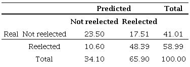
The classification table is frequently referred to as a confusion table. For
Garson (2011),
Although classification hit rates (percent correct) as overall effect size measures are preferred over pseudo-R
2 measures, they to have some severe limitations for this purpose. Classification tables should not be used exclusively as goodness-of-fit measures because they ignore actual predicted probabilities and instead use dichotomized predictions based on a cutoff (ex.: 0.50). For instance, in binary logistic regression, predicting a 0-or-1 dependent, the classification table does not reveal how close to 1.0 the correct predictions were nor how close to 0.0 the errors were. A model in which the predictions, correct or not, were mostly close to the .50 cutoff does not have as good a fit as a model where the predicted scores cluster either near 1.0 or 0.0. Also, because the hit rate can vary markedly by sample for the same logistic model, use of the classification table to compare across samples is not recommended. (
Garson, 2011, p. 173).
Our classification matrix uses the conventional standard of 50% to allocate cases as 1 (if the predicted probability is higher than 0.5) or 0 (smaller than 0.5). We can evaluate this table using three concepts: accuracy, sensibility, and specificity. The accuracy of the model is the proportion of true positive and true negative cases. According to
Table 9, the accuracy of our model was of 71.89% (23.50% + 48.29%). However, the accuracy of a model is not always the most important aspect. In certain cases, what is important is maximizing the rate of true positives or true negatives.
Moving on to sensibility. It is the percentage of cases that has the feature of interest (was reelected) that were accurately predicted by the model (true positives / false positives + true positives). In our example, 48.39% of reelected candidates were correctly classified, out of a total of 58.99% that were actually reelected. This gives us a sensibility of 82.03% (48.39%/58.99%). The specificity of the model is the percentage of cases that do not have the feature of interest (were not reelected), that were correctly classified by the model, that is (true negatives / false negatives + true negatives). As we can see, 23.50% of non-reelected candidates were correctly identified out of a total of 41.01% of non-reelected. This gives us a specificity of 57.30% (23.50%/41.01%). There is a trade-off between sensibility and specificity. When increasing one, the other diminishes. Although sometimes the sensibility of the model is more important (predicting an illness, since one would be able to treat it), at other times it is best to increase specificity (keep corrupt politicians from being elected).
VI. Conclusion
We hope to help students and teachers to better understand how logistic regression works. The absence of calculus, linear and matrix algebra, and advanced statistics limits our ability to understand more advanced data analysis techniques. For this reason, our approach focused on the intuitive exposition of results. We also believe that understanding the intuitive logic of logistic regression is the first step to better understanding the different procedures that exist to deal with categorical data. Computational advances allow researchers with less specific training in Mathematics and Statistics to benefit from the advantages associated with the different multivariate techniques. Given that many variables in Political Science are categorical, the analytical benefits associated with the correct application and interpretation of a logistic model are evident. With this paper, we hope to disseminate the use of logistic regression.
And how to improve the quality of methodological and technical training offered to Political Science undergraduate and graduate students in Brazil? We recommend the following: (1) incorporate of replication as a pedagogical tool in data analysis disciplines; (2) mandatory disciplines on mathematics, calculus, probability, and statistics in undergraduate and graduate curricula. In addition, students must receive training in some programming language; (3) conduct practical exercises involving data analysis with topics typical of Political Science. The emphasis onABSTRACT problems reduces students’ interests on the topic; (4) incentivize student participation in winter/summer courses such as MQ-UFMG and IPSA-USP; (5) promote epistemology and philosophy of science disciplines. The definition of research methods and techniques depend on the epistemological view of what is scientific knowledge and how it should be implemented; (6) diffuse critical reading of papers that use advanced data analysis techniques; (7) keep up with the academic production of journals specialized in methodology such as, for instance,
Political Analysis and
Political Science Research and Methods; (8) encourage the publication of methodological papers in national journals; (9) foster the creation of research groups and round-tables on methodology and data analysis techniques in professional conferences; (10) fund research projects especially devoted to deepening the knowledge on the main feature of science: method.
Appendices
Appendix
In this section, we present some information that can help researchers to interpret logistic regression coefficients. In particular, we examine the interpretation of the odds ratio. In addition, we list some learning tools.
• Understanding the odds ratio
32
The term odds ratio is not as disseminated in Political Science applied research as are mean or probability. Usually, since the researcher is comparing groups/categories, they are interested in analyzing which group/category has a better chance of occurring in relation to another group/category. Consider the following example: suppose that the probability (p) of a certain event occurring is 0,9. Thus, when calculating the complementary event, q = 1 – p, we have 1 – 0,9 = 0,1. Chance is the division of the probability of occurrence (p) by the probability of non-occurrence (q). Consequently, 0,9/0,1 = 9. It is stated, then, that the chance for success is 9 to 1. Alternatively, the chance for failure is 0,1/0,9 = 0,11. We say then that the chance for failure is 1 to 9. Unlike probability, which can only take on values between 0 and 1, chance can vary between 0 and infinity. When the probability of an event occurring is greater than the probability of it not occurring, its chance will be greater than 1. When the probability of it not occurring is greater, chance will be smaller than 1. When probabilities are equal (e.g., tossing a coin), chance is equal to 1. Given the pedagogical purposes of this paper, it is relevant to replicate the data from Schawb (2002), to better grasp this concept (
Table 1A).
Table 1A
Frequency
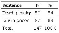
Table 1A shows that 34% of inmates were sentenced to the death penalty (n= 50/147). This means that the probability of this event occurring is 0f 0,34. Alternatively, the chance of being given capital punishment is 0,516 (50/97). Another way of saying this is that the chances are approximately half of being sentenced to capital punishment in relation to spending life in prison. Lastly, it is possible to invert the interpretation and consider life in prison roughly two times more likely than the death penalty.
So far, there are no independent variables. What the logistic model will inform is the impact of a given variable on the chance of a dependent variable occurring. For example, consider the relationship between race and sentence type (
Table 2A).
Table 2A
Sentence type by color
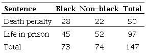
It is possible, then, to calculate the chance for each specific group: black people and non-black people. For black people, we have 28/45 = 0,622. For non-black people, we have 22/52 = 0,423. The impact of being black can be represented by the division of a black person receiving the death penalty and a non-black person receiving capital punishment (0,423). 0,622/0,423 = 1,47. For the interpretation: a) black people have 1,47 higher chance of receiving the death penalty than non-black people; b) being black increases by 47% the chances of receiving capital punishment (1,47-1*100).
Learning tools
http://www.icpsr.umich.edu/icpsrweb/sumprog/
Internationally, the
Summer Program in Quantitative Methods of Social Research (ICPRS) is one of the main initiatives in the dissemination of research methods and techniques.
http://www.fafich.ufmg.br/~mq/index.html
Intensive course in Quantitative Methodology in the Humanities. It is the most traditional course in teaching of research methods and techniques in Social Sciences in Brazil.
http://summerschool.ipsa.org/
Summer school organized by the International Political Science Association, the Department of Political Science, and the Institute for International Relations of the University of São Paulo (USP).
http://gking.harvard.edu/
Gary King shares papers on methodology, specific software, and databases for researchers interested in replication.
http://faculty.chass.ncsu.edu/garson/PA765/statnote.htm
David Garson presents different topics in multivariate statistics, using the Statistical Package for Social Sciences. At the end of each section, there is a suggested bibliography that can be used as reference to gain more in-depth knowledge on the topic.
http://www.statsoft.com/textbook/
Has different multivariate techniques using the software Stastistica.
http://www.ats.ucla.edu/stat/
Website for the University of California (UCLA) specialized in multivariate techniques. Here, the user finds applications for different software (SAS, SPSS, STATA, R, etc.), including video-classes and tutorials.
http://www.socr.ucla.edu/SOCR.html
At this address, the reader finds games, applications, analyses, among other tools related to teaching Statistics and different research techniques.
http://pan.oxfordjournals.org/
Political Analysis is one of the most influential journals in contemporary Political Science and publishes papers in the field of methodology.
http://www.amstat.org/publications/jse/
Journal specialized in the publication of teaching and learning techniques in Statistics.
http://www.politicahoje.ufpe.br/index.php/politica
The journal Política Hoje, from UFPE’s Department of Political Science, recently published a special issue dedicated to Methodology and Epistemology in Political Science and International Relations.
References
Altman, D. (1991) Categorising continuous variables.
British Journal of Cancer, 64(5), p. 975. DOI: 10.1038/bjc.1991.441
Bonney, G. (1987) Logistic regression for dependent binary observations.
Biometrics, 43(4), pp. 951-973. DOI: 10.2307/2531548
Brant, R. (1996) Digesting logistic regression results.
The American Statistician, 50(2), pp. 117-119. DOI: 10.2307/2684422
Castro, M.M.M. & Nunes, F. (2014) Candidatos corruptos são punidos?: accountability na eleição brasileira de 2006.
Opinião Pública, 20(1), pp. 26-48. DOI: 10.1590/S0104-62762014000100002
Codato, A.; Cervi, E. & Perissinoto, R. (2013) Quem se elege prefeito no Brasil? Condicionantes do sucesso eleitoral em 2012.
Cadernos Adenauer, 14(2), pp. 61-84.
Cohen, J. (1983) The Cost of Dichotomization.
Applied Psychological Measurement, 7(3), pp. 249–253. DOI: 10.1177/014662168300700301
Cook, R. & Weisberg, S. (1997) Graphics for assessing the adequacy of regression models.
Journal of the American Statistical Association, 92(438), pp. 490-499. DOI:10.1080/01621459.1997.10474002
R Core Team. (2019) R: A language and environment for statistical computing.
R Foundation for Statistical Computing. Vienna, Austria. Disponível em:
https://www.R-project.org/. Acesso em: 28 set. 2020.
DeMaris, A. (1995) A tutorial in logistic regression.
Journal of Marriage and the Family, pp. 956-968. DOI: 10.2307/353415
Eno, D. & Terrell, G. (1999) Scatterplots for logistic regression.
Journal of Computational and Graphical Statistics, 8(3), pp. 413-425. DOI: 10.1080/10618600.1999.10474822
Epstein, L.; Landes, W. & Posner, R. (2013)
The behavior of federal judges: a theoretical and empirical study of rational choice. Cambridge: Harvard University Press.
Fernandes, A.
et al. (2019) Why quantitative variables should not be recoded as categorical.
Journal of Applied Mathematics and Physics, 7(7), pp. 1519-1530. DOI: 10.4236/jamp.2019.77103
Figueiredo Filho, D.; Silva, L. & Domingos, A. (2015) O Que é e como Superar a Multicolinearidade? Um Guia Para Ciência Política.
Conexão Política, 4(2), pp. 95-104. DOI: 10.26694/rcp.issn.2317-3254.v4e2.2015.p95-104
Figueiredo Filho, D.
et al. (2019) Seven Reasons Why: A User's Guide to Transparency and Reproducibility.
Brazilian Political Science Review, 13(2), pp. e0001. DOI: 10.1590/1981-3821201900020001
Figueiredo Filho, D.; Silva Júnior, J. & Rocha, E. (2012) Classificando regimes políticos utilizando análise de conglomerados.
Opinião Pública, 18(1), pp. 109-128. DOI: 10.1590/S0104-62762012000100006
Fox, J. (1991)
Regression diagnostics: An introduction Vol. 79. Thousand Oaks, CA: Sage Publications.
Freitas, L. (2013)
Comparação das funções de ligação logit e probit em regressão binária considerando diferentes tamanhos amostrais. Tese de Doutorado. Viçosa: Universidade Federal de Viçosa.
Furlong, E. (1998) A logistic regression model explaining recent state casino gaming adoptions.
Policy Studies Journal,
26(3), pp. 371-383, DOI: 10.1111/j.1541-0072.1998.tb01907.x
Garson, G.D. (2014)
Logistic Regression: Binary and Multinomial. [s.l.]: Statistical Associates Publishing.
Goldsmith, B.; Chalup, S. & Quilan, M. (2008) Regime type and international conflict: towards a general model.
Journal of Peace Research, 45(6), pp. 743-763. DOI: 10.1177/0022343308096154
Guthery, F. & Binghan, R. (2007) A primer on interpreting regression models.
The Journal of Wildlife Management, 71(3), pp. 684-692. DOI: 10.2193/2006-285
Hagle, T. & Mitchell, G. (1992) Goodness-of-fit measures for probit and logit.
American Journal of Political Science, 36(3), pp. 762-784. DOI: 10.2307/2111590
Hair, J.
et al. (2009)
Análise multivariada de dados. Porto Alegre: Bookman Editora.
Henderson, E. & Singer, J. (2000) Civil war in the post-colonial world, 1946-92.
Journal of Peace Research, 37(3), pp. 275-299. DOI: 10.1177/0022343300037003001
Hilbe, J. (2009)
Logistic regression models. London: Chapman and Hall/CRC.
Hosmer Jr, D.; Lemeshow, S. & Sturdvanty, R. (2013)
Applied logistic regression Vol. 398. New York: John Wiley & Sons.
Hosmer Jr, D. & Lemeshow, S. (2000)
Applied Logistic Regression. New York: John Wiley & Sons.
Jaccard, J. & Jaccard, J. (2001)
Interaction effects in logistic regression. Thousand Oaks: Sage Publications.
Janz, N. (2016) Bringing the gold standard into the classroom: replication in university teaching.
International Studies Perspectives, 17(4), pp. 392-407. DOI: 10.1111/insp.12104
Kay, R. & Little, S. (1987) Transformations of the explanatory variables in the logistic regression model for binary data.
Biometrika, 74(3), pp. 495-501. DOI: 10.2307/2336688
Kennedy, P. (2005)
A guide to econometrics, Oxford: Maldon.
Keprt, A. & Snásel, V. (2004) Binary Factor Analysis with Help of Formal Concepts. In:
The Second International Conference on Concept Lattices and Their Applications (CLA). Ostrava, pp. 90-101. Disponível em:
http://ceur-ws.org/Vol-110/paper10.pdf. Acesso em: 13 out. 2020.
King, G. (1986) How not to lie with statistics: Avoiding common mistakes in quantitative political science.
American Journal of Political Science, 30(3), pp. 666-687. Disponível em:
https://ssrn.com/ABSTRACT=084228. Acesso em: 28 set. 2020.
King, G. & Zeng, L. (2001) Logistic regression in rare events data.
Political analysis, 9(2), pp. 137-163. DOI: 10.1093/oxfordjournals.pan.a004868
Kleinbaum, D. & Klein, M. (2010)
Logistic regression: A Self-Learning Text. New York: Springer-Verlag. DOI: 10.1007/978-1-4419-1742-3
Krueger, J. & Lewis-Beck, M. (2008) Is ols dead?
The Political Methodologist, 15(2), pp. 2-4, 2008.
Landwehr, J.; Pregibon, D. & Shoemaker, A. (1984) Graphical methods for assessing logistic regression models.
Journal of the American Statistical Association, 79(385), pp. 61-71. DOI: 10.1080/01621459.1984.10477062
Lewis-Beck, M. (1980)
Applied Regression. Thousand Oaks: Sage Publications.
Long, J. (1997) Regression models for categorical and limited dependent variables.
Advanced quantitative techniques in the social sciences, 7(s/n), Thousand Oaks: Sage Publications.
Lottes, I.; DeMaris, A. & Adler, M. (1996) Using and interpreting logistic regression: A guide for teachers and students.
Teaching Sociology, 24(3), pp. 284-298. DOI: 10.2307/1318743
Menard, S. (2000) Coefficients of determination for multiple logistic regression analysis.
The American Statistician,
54(1), pp. 17-24. DOI: 10.1080/00031305.2000.10474502
Menard, S. (2002).
Applied logistic regression analysis. Thousand Oaks: Sage Publications. DOI: 10.4135/9781412983433
Menard, S. (2004) Six approaches to calculating standardized logistic regression coefficients.
The American Statistician,
58(3), pp. 218-223. DOI: 10.1198/000313004X946
Nelder, J. & Wedderburn, R. (1972) Generalized linear models.
Journal of the Royal Statistical Society: Series A (General), 135(3), pp. 370-384. DOI: 10.2307/2344614
Nicolau, J. (2000) An analysis of the 2002 presidential elections using logistic regression.
Brazilian Political Science Review, 1(1), pp. 125-135.
O'Brien, S. M & Dunson, D. (2004) Bayesian multivariate logistic regression.
Biometrics, 60(3), pp. 739-746. DOI: 10.1111/j.0006-341X.2004.00224.x
O'Connell, A. (2006)
Logistic regression models for ordinal response variables. Thousand Oaks: Sage Publications. DOI: 10.4135/9781412984812
Pampel, F. (2000)
Logistic regression: A primer. Thousand Oaks: Sage Publications. DOI: 10.4135/9781412984805
Paranhos, R.; Figueiredo Filho, D.; Rocha, E. & Carmo, E. (2013) A importância da replicabilidade na ciência política: o caso do SIGOBR.
Revista Política Hoje,
22(2), pp. 213-229.
Pardoe, I. & Cook, R. (2002) A graphical method for assessing the fit of a logistic regression model.
The American Statistician, 56(4), pp. 263-272. DOI: 10.1198/000313002560
Pedhazur, E. (1982)
Multiple Regression in Behavioral Research. New York: Holt, Rinehart and Winston.
Peixoto, V. (2009) Financiamento de campanhas: o Brasil em perspectiva comparada.
Perspectivas: revista de ciências sociais, 35(s/n), pp. 91-116.
Press, S. & Wilson, S. (197) Choosing between logistic regression and discriminant analysis.
Journal of the American Statistical Association, 73(364), pp. 699-705. DOI: 10.1080/01621459.1978.10480080
Ribeiro, E.; Carreirão, Y. & Borba, J. (2011) Sentimentos partidários e atitudes políticas entre os brasileiros.
Opinião Pública, 17(2), pp. 333-368. DOI: 10.1590/S0104-62762011000200003
Roberts, G.; Rao, N. & Kumar, S. (1987) Logistic regression analysis of sample survey data.
Biometrika, 74(1), pp. 1-12. DOI: 10.2307/2336016
Schwab, J. (2002)
Multinomial logistic regression: Basic relationships and complete problems. Austin, Texas: University of Texas.
Soares, G. (2000) Em busca da racionalidade perdida: alguns determinantes do voto no Distrito Federal.
Revista Brasileira de Ciências Sociais, 15(43), pp. 5-23. DOI: 10.1590/S0102-69092000000200001
Speck, B. & Mancuso, W. (2013) O que faz a diferença? Gastos de campanha, capital político, sexo e contexto municipal nas eleições para prefeito em 2012.
Cadernos Adenauer, 14(2), pp. 109-126.
Stock, J. & Watson, M. (2015)
Introduction to Econometrics. 3ª Edition. United Kingdom: Pearson.
Tabachnick, B.; Fidell, L. & Ullman, J. (2007)
Using multivariate statistics. Boston, MA: Pearson.
Taylor, J. & Yu, M. (2002) Bias and Efficiency Loss Due to Categorizing an Explanatory Variable.
Journal of Multivariate Analysis, 83(s/n), pp. 248–263. DOI: 10.1006/jmva.2001.2045
Wong, G. & Mason, W. (1985) The hierarchical logistic regression model for multilevel analysis.
Journal of the American Statistical Association, 80(391), pp. 513-524. DOI: 10.1080/01621459.1985.10478148
Newspaper articles
Notes
Notes
1 Replication materials available at: <https://osf.io/nv4ae/>. This paper benefitted from the comments of professor Jairo Nicolau and the suggestions made by
Revista de Sociologia e Política‘s anonymous reviewers. We also thank the
Berkeley Initiative for Transparency in the Social Sciences and the
Teaching Integrity in Empirical Research.
2 For a brief review of Mensalão, see O julgamento do Mensalão (2012).
3 For a explanation of the Sanguessugas scandal, see Entenda o Escândalo dos sanguessugas (2006).
4 See the course on logistic regression offered by
Coursera (
https://www.coursera.org/course/logisticregression). We also suggest the categorical data analysis course given by the Intensive Training on Quantitative Methodology, from the Federal University of Minas Gerais (MQ – UFMG).
5 We will not discuss the mathematical foundations of logistic regression. For readers interested in the topic, we suggest Long (1977) and Pampel (2000).
6 There are extensions of the logistic model that enable modelling the variation of ordinal (ordinal logistic regression) and polychotomous variables (multinomial logistic regression).
7 Nelder and Wedderburn (1972) demonstrated that it is possible to use the same algorithm to estimate models of the exponential family, such as Logistic, Probit, Poisson, Gama, and Inverse Normal. Do not worry about the formulas for these models. The important thing is to understand what each of them are for, when they should be used, and how the coefficients must be interpreted.
8 Hair
et al. (2009) state that homoscedasticity is the assumption that the dependent variable displays equal levels of variance over a range of the predictor variable (Hair
et al., 2009, p. 83). 2013, p. 77
9 For Hair
et al. (2009), an implied assumption for all multivariate analysis techniques based on correlational measures of association, including multiple linear regression and logistic regression, is linearity (Hair
et al., 2009, p. 85).
10 One estimator is the
Best Linear Unbiased Estimator, when the following properties are satisfied. Best means efficient, producing the least variance, linear means the type of relationship expected between parameters, and unbiased concerns the sampling distribution of the estimator. A biased estimator is one that systematically over- or underestimates the value of the population parameter.
11 The data are available at: <http://www.ats.ucla.edu/stat/stata/examples/alr2/alr2stata1.htm>.
12 A logistic regression also supports variables with more than two categories. When there is no hierarchy between the category, such as with the distribution of civil status, we should use a multinomial regression. On the other hand, an ordinal logistic regression is ideal to model the distribution of ordinal variables, that is, when there is a structure of intensity between the categories.
13 Categorizing variables tends to produce biased and inefficient estimates (Taylor & Yu, 2002). Given this, we emphasize the term “originally dichotomous”, and recommend never reducing the level of measurement for continuous, discrete, or ordinal variables with the aim of applying logistic regression models. Still in doubt? Check Fernandes
et al. (2019).
14 When the correlation is very high (some use the golden rule of r ≥ 0,90), the coefficients’ standard error is large, hindering the evaluation of the relative importance of the explanatory variables. To better understand the problems that high levels of correlation among independent variables may generate, see Figueiredo, Silva, and Domingos (2015).
15 For an introduction on how to detect outliers, see Figueiredo Filho and Silva (2016), available at: <https://cienciapolitica.org.br/system/files/documentos/eventos/2017/04/outlier-que-pertuba-seu-sono-como-identificar-e-manejar.pdf>.
16 A researcher may provide the data at Harvard University’s
Dataverse. The
Open Science Framework may also be used to make available data for broader projects. In Brazil, we suggest the Social Information Consortium (CIS).
17 In a linear model, the regression coefficient is represented as the variation observed on the dependent variable (Y) when the independent variable (X) increases in one unit. In a logistic regression, the coefficient indicates the variation in the logarithm of the chance for the dependent variable by increasing the explanatory variable in one unit.
18 Readers unfamiliar with the concept of chance should consult the Methodological
Appendix of this article before reading further. For a more detailed treatment, see
Hilbe (2009).
19 When interpreting the statistical significance of the confidence interval of the odds regression coefficient, we must observe if the interval includes the value one (1). If so, we are faced with a non-significant result. For example, in a confidence interval in which the coefficient varies between 0,8 and 1,6, it is not possible to reject the null hypothesis.
20 Following best scientific practices, the authors made the data and scripts available at the following website: <http://thedata.harvard.edu/dvn/dv/felipenunes>.
21 The main advantage of using 0/1 coding is that the distribution’s mean will be equal to the proportion of 1 cases in the sample. In a distribution with 100 occurrences, in which 25 cases have been coded as 1, the mean will be 0.25, which represents exactly the proportion of events coded as 1.
22 Castro and Nunes (2014) estimated the regression model from a probit link function. The logit function is better suited for small samples (n < 20) given that it presents a higher convergence rate. For large samples, on the other hand, there are no significant differences among these link functions. For more information on the topic, see Freitas (2013).
23 The researcher must make sure that no category has a distribution smaller than 5%. This is due to the phenomenon being then categorized as rare, and specific corrections to deal with this situation are needed. For interested readers, see King and Zeng (2001).
24 These finds diverge residually from the information reported in Tables 4 and 5 by Castro and Nunes (2014), which indicate 9 reelections out of a total of 50 representatives, equaling 18%.
25 And this can be calculated from the odds ratio, which is calculated by the dividing the chances of reelection for each group, in this case, 1.9/0.22. That is, candidates not involved in corruption scandals have an 8 times higher chance of being reelected when compared to the deputies named in the Mensalão and/or Sanguessugas schemes, as measured by Castro and Nunes (2014).
26 For Garson (2011), the omnibus test can be interpreted as a test for the joint capacity of all the predictors in the model to predict the response (dependent) variable. A significant result indicates that the fit is adequate to the data, suggesting that at least one of the predictors is significantly related to the response variable.
27 In the original, “the successful allocation of pork does not present, subverting expectations, positive association with reelection. The result seems to be null and irrelevant to explain the chances of reelection in 2006, also when socioeconomic and institutional variables are included in the model”. (Castro & Nunes, 2014, p. 42).
28 The maximum likelihood method is an iterative process that aims to fit the model through several repetitions. However, sometimes the model simply does not converge. This can happen for several reasons, from problems in the algorithms uses to estimate the link function to a strongly asymmetrical distribution of the independent variables.
29 There is a debate on the advantages and limitations of R
2 as a synthetic measure to evaluate the quality of fit of logistic regression models. To our knowledge, King (1986) is the first systematic alert on the issue in empirical research in Political Science. Figueiredo Filho, Silva Júnior, and Rocha (2012) have a pedagogical discussion on the topic.
30 Hair
et al. (2009) state that a logistic model’s fit can be evaluated by two main procedures: (1) pseudo R
2s, similarly to a linear regression and (2) by estimating the predictive capacity of the model.
31 There are also McFadden's pseudo R
2, McKelvey and Savoina pseudo R
2, McFadden pseudo R
2, Cragg and Uhler pseudo R
2 and Efron pseudo R
2. For the reader interested in deepening their knowledge on the subject, see Hagle and Mitchell (1992) and
Menard (2000).
32 This section was based on Schwab (2002).
A produção desse manuscrito foi viabilizada através do patrocínio fornecido pelo Centro Universitário Internacional Uninter à
Revista de Sociologia e Política.
Author notes
Antônio Alves Tôrres Fernandes (antonio.alvestorres@ufpe.br) is a master’s student in Political Science in the PPGCP/UFPE, an undergraduate student in Economics (UCB/DF), and a member of the Research Methods in Political Science Group (DCP/UFPE).Dalson Britto Figueiredo Filho (dalson.figueiredofo@ufpe.br) is professor at Political Science Graduate Program at Federal University of Pernambuco and author of the book “Quantitative methods in Political Science”, Editora InterSaberes.Enivaldo Carvalho da Rocha (enivaldocrocha@gmail.com) is a retired full professor at Political Science Graduate Program at Federal University of Pernambuco.Willber da Silva Nascimento (nascimentowillber@gmail.com) holds a PhD in Political Science from UFPE and works as postdoctoral researcher at PPGCP/UFPE/FACEPE.
