INTRODUCTION

In Physical Geography, notable that landscape units in different locations may have similar structural characteristics. The typologies that classify these units (ISACHENKO, 1991) are created through theoretical generalizations. A typology is a classification system (taxonomy) of landscapes’ structure, based on similar elements with a characteristic spatial dimension, grouped utilizing defined criteria, which may or not be subordinate.

Typology allows geosystems to be distinguished by their similarity (homogeneity) and repetition (spatiality) and has become essential in the study of landscapes. According to Rodriguez and Silva (2019,p.34), the classification of subdivisions is essential to understanding landscapes. At present, it is based on morphological and functional indicators and the subdivision of geosystems. The construction of a typology is based on the principles of analogy, homogeneity, replication, belonging to the same group, and the existence of areal discontinuities between their boundaries. From the perspective of multiscale analysis, the creation of a typology can take place in two ways (Figure 1), as highlighted by Cavalcanti and Corrêa (2013, p.153, emphasis added):

_{Multiscale analyzes can still be classified by hierarchical detection. Starting from a large geographical scale towards smaller scales is a downscaling or top-down approach. Starting from small geographical scales towards larger scales is an upscaling or bottom-up approach.}

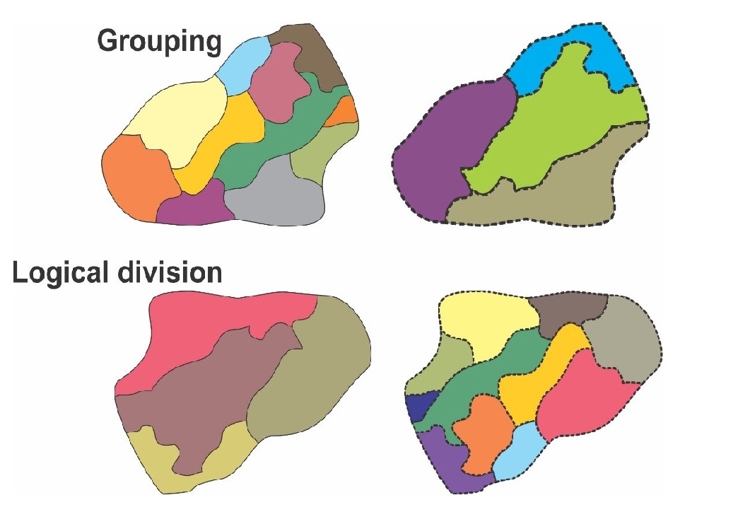
Figure 1
Grouping and logical division for landscape classification.
Braz, Salinas Chávez, and Oliveira (2019).

Classification is a complex process, which can involve a large number of elements that make up landscapes. In this context, a possible approach is statistical grouping (clustering) that creates models of associations of variables, with high numbers of landscape units¹

The precise objective of this work is to carry out a comparative assessment of different forms of grouping (clusters) to establish a landscape typology for the municipality of Mineiros, in the state of Goiás, Brazil, supported by the following factors: morphostructure, geology, geomorphology, altitude, slope, drainage density, soils, and land use and cover.

THEORETICAL REFERENCES

Representations of landscape syntheses use at least three approaches through a taxonomicclassification system: typology, regionalization, and topology. This makes it possible to create landscapev unit maps on different scales and in different conditions (environmental and territorial), as part of thelandscape cartography.

As well as providing a spatial representation, they can show groupings of individuals (thedelimitation of spatial sets in homogeneous zones) characterized by groupings of attributes or variablesthat are commonly understood through different landscape units (ZACHARIAS, 2008; SALINASCHÁVEZ et al., 2019).

The concept of typologies emerged through Berg’s zonality principles (1947) and continues todevelop today through the application of multivariate analyzes, which are considered a fundamental stepin the definition and logical treatment of landscapes’ sectoral parameters (BERUTCHACHVILI andBERTRAND, 1978).

Typology involves the classification of landscapes according to their structure and consists ofhomogeneous (similar) elements based on the interests and the scale of analysis of the study in question.According to Rodríguez and Silva (2002, p. 98), “Typology means distinguishing units by theirsimilarity and repetition, depending on certain homogeneity parameters”.

Bolòs i Capdevila (1981) suggests that the classification of geosystems consists of specifying thesimilarities (homogeneities) between individuals to group those that have possible identities into a taxon.Therefore, a taxon is a set of individuals, in this case, geosystems, which have a high degree ofsimilarity. The different taxa can also be grouped in other levels (higher or lower).

The head of the Siberian Institute of Geography, Sochava (1970; 1975; 1978a; 1978b) led thecreation of a taxon chorological system for landscape classification. This system is organized in abilateral row containing geomers, geosystems with a homogeneous structure, and geochors, geosystemswith a differentiated structure. Even so, Sochava (1978b, p. 8) highlights that “no classification isabsolute; it is necessary to modify it, improve it ”.

The hierarchical approach, widely discussed by Klijn (1995), led the author to consider that thepredominant principle of a hierarchy is that its elements must be based on inequality in theirrelationships. In the hierarchy of landscapes, it is possible to adopt the relationships established by Klijn(1995), regarding homogeneity or heterogeneity, symmetry, and asymmetry, respectively (Figure 2).

Figure 2
Symmetrical (homogeneous) and asymmetric (heterogeneous) relationships in hierarchies. 1)“A” dominates “b”, unilaterally; 2) “A” dominates “b”, but “b” affects “A”; 3) “A” and “b” affect eachother similarly.

This system of hierarchizing geosystems presupposes the grouping of landscapes in units ofdifferent classes, scales, or taxonomic levels. It is common practice for taxonomic levels to have aparticular designation: species, genus, and types of landscapes, among others, according to theirstructural, genetic, or functional specificity. The landscapes’ predominant and most important propertiesare established using this process of typological classification (taxonomy) (BAYANDINOVA,MAMUTOV, and ISSANOVA, 2018; SERRANO GINÉ et al., 2019).

With the advent of geoinformation, the use of Geographic Information Systems (GIS) has givennew impetus to mapping techniques for landscape units. This is exemplified by Isachenko and Reznikov(1995), who state that

_{It is easily verified that, even for a small territory in the taiga zone, there may be dozens of possible dynamicscenarios for the landscapes. It is impossible to map by traditional manual methods. Therefore, future steps onthe path of landscape modeling will be connected with the possibilities of GIS technologies (ISACHENKOand REZNIKOV, 1995, p. 804, our translation).}

Given the possibility of modeling for mapping landscapes, the use of statistics can also contributeto this task. According to Preobrazhenskiy (1983), in the mid-1970s, the first studies to consider such apossibility were by Aleksandrova (1975), who used automated techniques to evaluate landscapes fromthe correlation of a geographic, mathematical, and statistical model.

Shortly afterward, Kuprianova (1977) analyzed the geographical correlation of the naturaldifferentiation of the regionalization of landscapes, by applying computerized and automatic proceduresto complex objects (PREOBRAZHENSKIY, 1983).

PROCEDURES

The following eight elements were used to start the mapping: morphostructure, geological units,relief, hypsometry (altitude), slope, drainage density, soils, and land use and cover (Table 1).

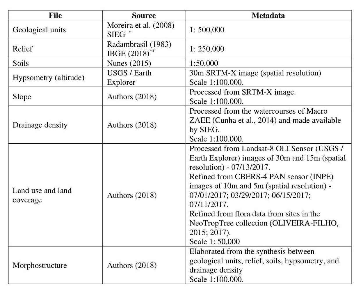
Table 1
Characteristics of the data used
Authors, 2018.

The crossing of elements using vector data (shapefiles) resulted in a file with 67,691 features. Theresearch steps are summarized in the flowchart in Figure 3.

The result was converted to a given raster (.tiff), reclassified, and submitted to fuzzy(fuzzification) logic. In this conversion process, the raster admits 245 intervals (the binary logic of an8-bit raster allows a maximum of 255 intervals).

_{The diffuse classification [fuzzy logic] assumes the limit between two neighboring classes as a continuousoverlapping area in which an object participates partially in each class. This point of view not only reflects thereality of many applications in which categories have diffuse boundaries, but it also provides a simplerepresentation of the potentially complex partition of the resource space (ZHENG and KAINZ, 1999, p. 79).}

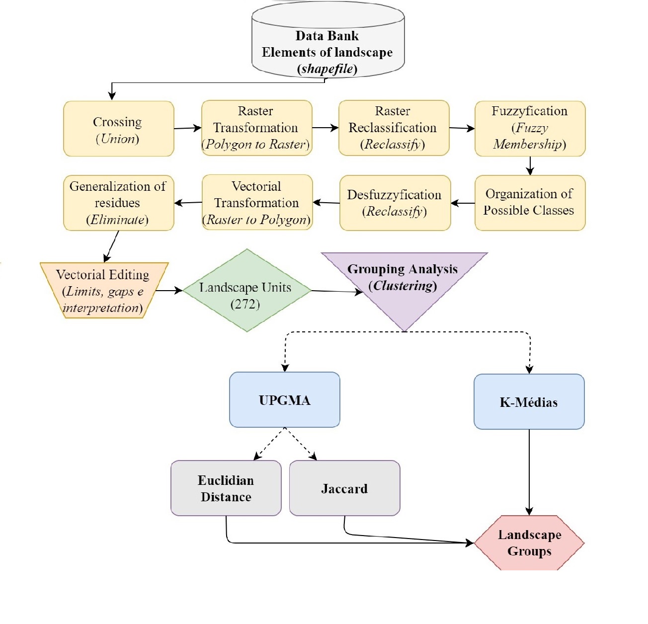
Figure 3
Flowchart of the procedures for grouping landscape units.
Authors (2019).

In the context of landscape cartography, fuzzy logic is mainly relevant in defining geosystems’limits because, according to Marques Neto (2016), the boundaries between landscapes can be abrupt andwell-marked, but they can also change from one unit to another in a diffuse and interdigitated way thatmay make adequate and more accurate cartographic representation impossible.

The next step was the defuzzification of the raster and its transformation into a vector (shapefile)to deal with the residues and correct the confusions in the grouping or separation of possible landscapeunits, based on cartographic generalization, opting for a cartographic area of at least 5ha.

As specified by Salinas Chávez and Ramón Puebla (2013), the minimum cartographic area of 5 hacorresponds to cartographic representations on the scale of 1: 50,000. After the necessary adjustments,the 245 classes were manually reorganized (vectorization), revised and finally, 272 landscape units wereobtained for the municipality of Mineiros (GO).

The map of landscape units - and subsequently of landscape groups - is represented on a scale of1: 100,000, to value the landscape differences (by a principle of homogeneity2). For the proceduresdescribed above, the geoinformation was organized in a Geographic Information System (GIS), usingthe ArcGIS 10.4.1 software.

Due to the large number of landscape units (272), it was necessary to create groups (clusters) thatwere similar. This is a common statistical technique when large amounts of numbers are involved. Italso resembles the principles of mapping landscapes, which aim to determine elements withhomogeneous structures, and those that are heterogeneous, identifying different hierarchies of “clusters”or “separations” and finally, simplifying their cartographic representation.

The typology was performed through cluster analysis (clustering), by applying multivariatestatistics. This procedure was adopted because of the number of observation objects. In this way, effortswere concentrated on grouping these units into higher hierarchies with a certain degree of similarity to represent groups of landscapes through clustering.

The cluster analysis (clustering) was carried out using the PAST statistic (3.25), software and theUnweighted Pair Group Method with Arithmetic Mean - UPGMA method was selected, using theEuclidean and Jaccard Distance similarity coefficients and the K-means algorithm.

The UPGMA calculates the average distances or similarities between a landscape unit (LU) andeach of the other LUs, which all receive the same weight, with the matrix (of distance or similarity)being updated and reduced at each stage of the algorithm. It is, therefore, an agglomerative (bottom-up)strategy (LEGENDRE and LEGENDRE, 2012).

Concerning the application of the UPGMA, Metz (2006, p.23) points out that

_{this approach, like the others, builds the groupings so that examples belonging to the same cluster have highsimilarity and examples belonging to different clusters have a low similarity. [...] However, a distinctionbetween this approach and the others is that the result obtained is not just a partition of the initial data set, buta hierarchy that describes a different partitioning at each level analyzed.}

Regarding the coefficients used in this work, it is notable that the Euclidean distance, which was“defined by the Greek mathematician Euclides and represents the shortest distance between two objectsin the multidimensional plane” (MACHADO, 2011, p. 29), is the most common metric distance used incluster analysis (clustering), as explained by Metz (2006), and defined by Equation 1 below:

(1)
(1)

The Jaccard coefficient (JACCARD, 1901) is a similarity metric, understood as a coefficient usedto measure association when the characteristics are only described by two discrete values, for example, 1or 0. The Jaccard coefficient considers that the correspondence between the 0-0 (non-existent) values isless important than that of the 1-1 (existing) values. This occurs because, in most applications, the value1 is used for attributes where the described characteristic is present and the value 0 indicates the absenceof the characteristic (Equation 2) (METZ, 2006). “Thus, this algorithm compares the number ofpresences of common variables and the total number of variables involved, excluding the number ofjoint absences” (MEYER, 2002, p. 9).

(2)
(2)

As well as using a hierarchical algorithm (UPGMA), a non-hierarchical and non-supervisedK-means algorithm was used. Initially, the clusters are assigned randomly. Then an iterative procedureis adopted, where items are moved to the cluster with the closest average to the grouping. The procedureis repeated continuously until the items are not closer to other clusters (HAMMER, 2019).

The k-means proposed by MacQueen (1967), is heuristic, as an algorithm takes two propertiesinto account when creating its structure. Furthermore, k-means is considered an unsupervised clusteringalgorithm because it generates groupings from predetermined class numbers. The k-means has a rapidexecution time, based on strategies to make simple and fast choices, iteratively minimizing the elements’distance to a set of k-centers given by x = {x1, x2, ..., xk}. The k-means depends on a parameter (k =number of clusters), which is pre-established by the user. This is a non-hierarchical algorithm, given byEquation 3 (LINDEN, 2009):

(3)
(3)

Operationally, the construction of the typology appropriated the 272 units and each of the 71classes of the eight elements used for mapping the units, organizing them in a “presence-absence” binarymatrix - assigning 0 to elements absent in the landscape unit and 1 for elements present in the unit. Thisprocedure defines the similarities or differences between the input elements from a distance, in this case,the Euclidean distance or similarity coefficient. Linden (2009, p.18-19) highlights that

_{The criterion is usually based on a dissimilarity function, which receives two objects and returns the distancebetween them. [...] Groups determined by a quality metric must have high internal homogeneity and highseparation (external heterogeneity). This means that the elements of a given set must be mutually similar and,preferably, very different from the elements of other sets (LINDEN, 2009, p. 18-19).}

Thus, the 272 landscape units were grouped into landscape groups, using the UPGMA (EuclideanDistance and Jaccard) procedure resulting in a dendrogram, formed by the grouping of landscape units atlevels of distance from the clusters formed. However, the K-means results directly in a matrixcontaining the intervals of the clusters.

To validate the groupings, it was assumed that the sixteen types of landscapes constitute thereality in the field, considering that even products generated from the cluster were manually refinedthrough the fieldwork.

Therefore, the validation involved selecting two well-known locations that had been extensivelyverified in the field, which were compared with the limits of the landscape types, field validation points,and with each of the groupings resulting from the UPGMA and K-means.

In addition to the manual measurement, based on field information, statistical tests for the clusterswere included, using the MATLAB, “evalclusters” with the Silhouette, Davies-Bouldin, and Gap indices.

RESULTS AND DISCUSSION

The crossing of the elements defined 272 landscape units. Although at first, this situation isindicative of the diversity of landscapes in the municipality of Mineiros (GO), from the point of view ofcartographic representation and the intention to use the landscape information for environmental andterritorial planning, it was deemed necessary to adopt other (geographic and cartographic) analysis scales³.

The issue of geographical scale in the study of landscapes is very relevant since in Sochava’stheory of geosystems (1978a) the author was already pointing to the bilateral rows of geomers andgeochores, as well as their suborders and subcategories4. Solntcev (1949; 2006) had also raised concernsabout the delimitation of landscape units, both in terms of geographic and cartographic scales, and thenumber of units to be represented, due to their analytical complexity.

The groupings using the unweighted pair group method with arithmetic mean - UPGMA resultedin dendrograms, whose intervals on the cut lines were 3.0 for the Euclidean distance, and 0.25 forJaccard (Figure 4).

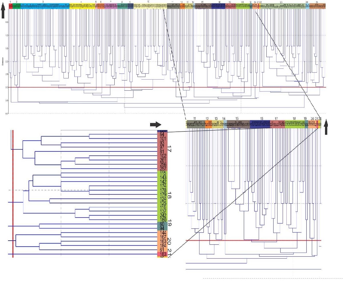
Figure 4
Dendrogram resulting from the UPGMA cluster analysis (Euclidean distance).
Authors (2019).

It is essential to emphasize that each mapping reality has particularities regarding the distinctionof the landscape units; there is no inflexible rule when selecting cut lines that are always the same in theresulting dendrograms. However, the choice of cut lines directly impacts the quantity and configurationof the landscape units’ boundaries (Figure 4).

As regards the UPGMA grouping, the determination of its quality occurs from the evaluation ofthe co-phenetic correlation coefficient, with 0.7425 for the Euclidean distance and 0.759 for Jaccard.According to Rohlf’s (1970) proposal, co-phenetic correlations > 0.7 are permissible for goodgroupings.

The result for the k-means is given directly by a matrix indicating the groups (clusters) of therespective landscape units (Table 1).

Table 2
Matrix resulting from the cluster analysis by k-means.
Authors (2019)

The clusters are then organized according to the landscape units and used to map the landscapegroups (Figure 5).

The manual procedure was selected to assess the clusters, anchored in field information andstatistical evaluation, based on cluster validation indexes. Gath and Geva (1989) and Silva and Gomide (2004) specify at least three requirements when defining an acceptable grouping, namely: 1) the clearseparation between the resulting groups; 2) a certain concentration (cohesion) of points around thecenter of a group; and 3) the smallest possible number of groups, provided that they also comply withthe previous requirements.

However, there is a need for caution when dealing with groupings involving spatial limits, since itis clear that, in this case, statistical significance does not take spatial significance into account, despiteits great importance for landscape cartography.

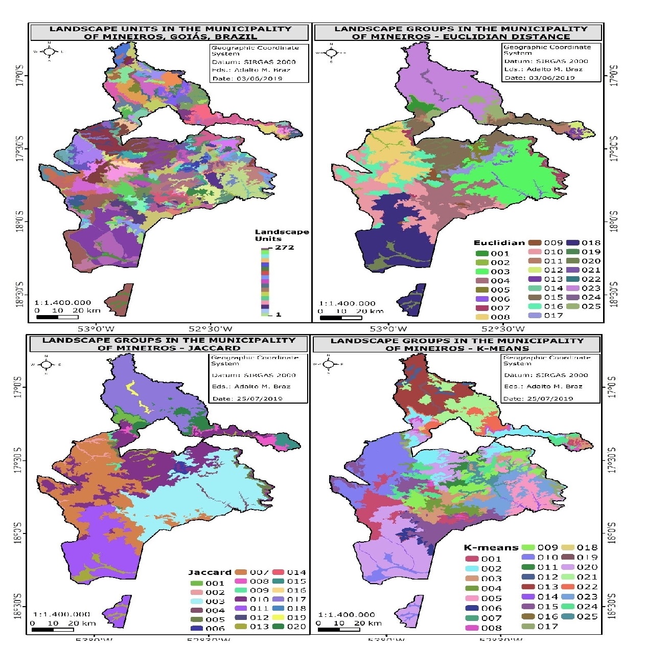
Figure 5
Map of landscape units and landscape groups by Euclidean distance.
Authors (2019).

The results of the manual validation indicated that in terms of reliable groupings, the hierarchicalmethod, in this case, the UPGMA algorithm, proved to be more advantageous than the k-means when considering the limits of the landscape types and the landscapes of Mineiros in particular. The validation(Figure 6) adopted three better-known field areas and concentrated the measurement points, to comparewith the landscapes and landscape types identified in the field activities.

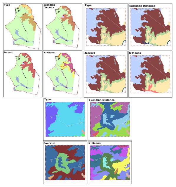
Figure 6
Validation of clusters in each algorithm and similarity metric of the cluster to the south(Emas National Park), north (Pinga-Fogo), and center of the municipality of Mineiros, Goias, Brazil

⁽⁵⁾

The statistical validation employed the Silhouette, Davies-Bouldin, and Gap indices, which assessthe ideal number of clusters. The Silhouette index gave the best cluster result with the Jaccardcoefficient and the k-means of twenty-five groups. The Gap index indicated the most satisfactory clusterusing the UPGMA algorithm, applying the Euclidean distance similarity metric (corroborating themanual assessment for the landscape limits), followed by the k-means of twenty-five groups. Althoughthe Davies-Bouldin metric showed the ideal grouping of k-means of 25 groups, this index was unable tospecify similarity metrics (except Euclidean and Jaccard distances), therefore, its results were discardedfrom the assessment.

For the clustering procedure using the Euclidean distance, there was a cut line of 25 groups oflandscapes, whereas, with Jaccard, the choice of the cut line indicated 20 groups. For the k-means, the earlier choice of 25 groups of landscapes was opted for.

The main difference in the mappings is in the spatial limits of the resulting landscape groups. TheJaccard grouping created more extensive groups, which tended to be regulated by the formations of therelief, lithology, and morphostructure of the municipality.

Although like Jaccard, it conserved some larger landscape groups, the Euclidean distance resultedin a set of spatial limits that were more coherent and better suited to the desired mapping scale (1:100,000). As a result, it is considered to be the most appropriate, specifically for the interests proposedin this work.

Even though it had the same number of landscape groups as the Euclidean distance, in thek-means grouping there was a greater fragmentation in the spatial limits, and it was not possible to pointto one of the elements (soil, relief, etc.) as a regulator in the landscape groups.

Thus, it is understood that both the issues of scale and spatial significance are very relevant in thestudy of landscapes, and they should be considered with the same weight attributed to the clusteringprocedures and their statistical significance.

With traditional manual procedures, the grouping should be carried out analytically in each of 272landscape units, correlating them from their structural elements (relief, soil, vegetation, etc.) and seekingcorrespondence with analogous (homogeneous) units.

However, the software algorithms indicate which objects (landscape units) have analogouselements in their structure. When modeling the data in a quantitative (statistical) way, the softwareindicates different grouping levels of landscape units. The clustering levels defined by the cut linessuggested by the dendrogram, in the case of Euclidean and Jaccard distance, or the resulting k-meansmatrix, also suggest different geographical scales for landscape analysis.

Although the contribution of cluster analysis for the grouping of landscapes has been recognized,some questions can still be raised.

The first involves considering how the spatial significance between the landscape units from thegroupings suggested by the cluster classification can be obtained since the statistical significance(cluster) does not take the spatial significance of the landscape units’ boundaries into account.

Another reflection involves the capacity of the statistical technique (clustering) to determine thepreponderant elements in the landscape groupings. For example, is geomorphology, in fact, the mainelement that conditions the formation of landscape groups? This situation leads to another observation:is it possible to identify possible elements that condition the landscape groups from the cluster analysis?

One of the most relevant issues in landscape cartography is geographical and cartographic scale.Given this, the UPGMA (Euclidean and Jaccard distance) cluster analysis indicates the cut lines, whichdifferentiate the levels of the resulting clusters.

Therefore, the issue involves finding a relationship between the grouping levels (cut lines) and thegeographical and/or cartographic scales that are representative of the complexity (and reality) of therepresentation of the landscapes. Or, in the case of k-means, the same relationship with the number ofclusters predetermined by the user.

Assuming that in this case, the most relevant grouping was the Euclidean distance, initially, therewas no rule, or even a trend, in the genetic sense of conditioning the landscapes that indicated aregulation in the formation and hierarchy of geosystems. Thus, when considering the three groupingtechniques (Euclidean distance, Jaccard, and k-means) there was no consensus in identifying one ormore preeminent elements in the formation or even the grouping of landscapes

Reflection on the results presented, reinforces, for the time being, the premise that in theorganization and formation of landscapes all the structure’s elements are interrelated. The grouping,therefore, followed the premise of one of the theoretical-conceptual models of landscapes, corroborating Sochava’s (1978, p. 292) definition that geosystems are “a dimension of terrestrial space where thedifferent natural components have systemic connections with each other, with a defined integrity”.Consequently, the study results were considered satisfactory, with the attributes used exerting adecentralized influence on the formation of landscape units.

The statement that there were “gains” and “losses” in each similarity algorithm and metricadopted is very relevant to the results. Even so, the Euclidean distance, through the UPGMA algorithm, was the metric that came closest to reality (types of landscapes and reality in the field). There is also theassertion that the Jaccard metric can also be considered adequate for landscape groups, consideringsome “gains” and “losses” in the representation of landscape groups⁶ .

The k-means (with 25 landscape groups) is the least satisfactory algorithm as its grouping hadmore “losses” in the representation of the reality of the landscapes, especially in relation to theboundaries of the types of landscapes in the municipality of Mineiros (GO).

CONCLUSIONS

The use of clustering is a differential technique and still little explored in works in the field ofPhysical Geography, especially in Brazil, but it has shown considerable potential in landscape unitgroupings for cartographic representation.

The use of clustering statistical techniques was relevant for the optimization of processes. Evenso, it is noteworthy that this is an option to subsidize the mapping of landscapes but given what has beenpresented and discussed in this work it cannot be understood as the main and indisputable orientation inthe definition of landscape units. As already presented, there is a need to differentiate statisticalsignificance from spatial significance within the limits presented by the landscape clusters.

The procedure’s biggest advantage was that it optimized the regrouping of the unit limits forlandscape groups. So, based on the Euclidean distance clustering optimized 91% of the limits betweenthe 272 landscape units and their grouping into 25 landscape groups, in a very short time.

Hence, the relevance of this technique is its contribution to clustering procedures, that is, itgrouped and redefined a large amount of information that would be excessively slow using manualanalysis and spatial regrouping.

Specifically regarding the cluster algorithms, validating Linden’s premises (2009), it wasidentified that the k-means tends to emphasize homogeneity and ignore quality in the separation ofclusters, which in this research may justify the fragmentation in the spatial limits of landscape groupsand, consequently, the reduced spatial significance.

Another weakness of the k-means is the problem of the prior selection of the number of clustersby the user since it is not usually known a priori exactly how many clusters will be ideal, which mayinduce the arrangement of the resulting landscape groups. Linden (2009) also pointed out that a smallnumber of clusters may perhaps merge two “natural” clusters, while a larger preselected number willinfluence an exaggerated break up of “natural” clusters.

The hierarchical cluster algorithms tested through UPGMA, Euclidean distance, and Jaccard havethe advantage of results that not only differentiate the clusters but also identify the structure and thecontext of grouping the landscape units, through the dendrogram. Thus, it is possible to choose differentgrouping levels - in a possible relationship with the desired scale, in the case of landscapes - and obtainthe grouping hierarchy more comprehensibly.

As a result, it is possible that the choice of intervals (cut line in the dendrogram) may also imply,a form of “preselection” of landscape groups. Unlike the k-means, it is not a preceding choice, but it isstill a decision that will impact the number of groups obtained.

Currently, this is considered a weakness of the UPGMA, in terms of determining which cut line toadopt in different situations and objectives in landscape cartography. This leads us to question whetherthe cut line should only be adopted to evaluate the number of landscape groups to be represented later.

Regarding the results of the statistical validation, the indexes aim to evaluate the ideal number ofclusters. Even so, this analysis is not entirely sufficient to determine the best cluster for landscapegrouping, considering that the k-means was the least satisfactory algorithm for the grouping and themost acceptable from the point of view of the ideal number of clusters. The Gap index, in turn,corroborated the choice of Euclidean distance as the best similarity metric for grouping landscapes.

The Silhouette index pointed to Jaccard as a satisfactory metric of similarity, confirming thatJaccard would be an acceptable metric for adopting the cluster to group landscapes, evaluating the“gains” and “losses” of their results for the representation of landscapes.

Consequently, the results broaden the spectrum on the perspectives that can still be explored onthis theme, through new analyzes that aim to overcome existing challenges, such as:

To improve the assertion on the grouping levels (cut lines) and their possible relationship with thegeographical and/or cartographic scales, aiming at greater rigor in the cartographic representation oflandscapes in parallel with reality.

To understand which elements would be preponderant in landscape grouping, that is, which ofthem would condition the formation of some landscape groups.

The complexity of concomitantly obtaining the statistical and spatial significance between thegroups suggested by the statistical clustering analysis.

The urgency of carrying out future tests and comparisons with other non-hierarchical algorithmsand metrics, such as Principal Component Analysis - PCA, taking into account that k-means was theleast satisfactory algorithm and the only non-hierarchical method tested.

ACKNOWLEDGMENTS

The first author is grateful to the Coordination for the Improvement of Higher EducationPersonnel (CAPES) for the Ph.D. Social Demand scholarship and the International Association ofLusitanists (AIL) for the Scholarship for Young Researchers at the University of Coimbra (UC).

The other authors would like to thank the National Council for Scientific and TechnologicalDevelopment (CNPq) for financing the projects “Cartography of tourist landscapes of Brazilian andMozambican savannas” and “ The influence of relief on the structuring of landscapes in differentbiomes”.

All the authors thank Dr. Rosana Veroneze, a postdoctoral researcher linked to the Faculty ofElectric Energy and Computing (FEEC) at Unicamp, and Dr. Jean Metz, Machine Learning andSoftware Engineer at the company JArchitects (Belgium), for their assistance in carrying out the clusterstatistical validation and for their clarifications on the indexes.

REFERENCES

ALEKSANDROVA, T. D. Statistical methods of study of natural complexes. Moscow: Nauka, 1975. (Em russo)

BAYANDINOVA, S.; MAMUTOV, Z.; ISSANOVA, G. Man-made ecology of East Kazakhstan. Singapore: Springer Nature, 2018.

BERUTCHACHVILI, N.; BERTRAND, G. Le géosystème ou «système territorial naturel». Revue géographique des Pyrénées et du Sud-Ouest, Toulouse, vol. 49, n. 2, p. 167-180, 1978.

BOLÒS i CAPDEVILA, M. Problemática actual de los estudios de paisaje integrado. Revista de Geografía, Barcelona; v. 15, n. 1-2, p. 45-68, jan./dez., 1981.

BRAZ, A. M.; OLIVEIRA, I. J.; SALINAS CHÁVEZ, E. Agrupamento estatístico (cluster) para a determinação hierárquica de unidades tipológicas de paisagens. In: ENCONTRO NACIONAL DA ANPEGE, 13., 2019, São Paulo. Anais... São Paulo: ANPEGE; USP, 2019. p. 1-14.

CASTRO, I. E. O problema da escala. In: CASTRO, I. E.; GOMES, P. C. C.; CORRÊA, R. L. Geografia: conceitos e temas. 2. ed. Rio de Janeiro: Bertrand Brasil, 2000. p. 117-140).

CAVALCANTI, L. C. S.; CORRÊA, A. C. B. Problemas de hierarquização espacial e funcional na ecologia da paisagem: uma avaliação a partir da abordagem geossistêmica. Geosul, Florianópolis, v. 28, n. 55, p 143-162, jan./jun. 2013.

CUNHA, J. G. et al. (Coord.). Macrozoneamento Agroecológico e Econômico do Estado de Goiás. Um novo olhar sobre o território Goiano. Produto I: Sistematização de dados existentes em uma base de dados georreferenciada em ambiente de Sistema de Informações Geográficas (SIG) e suporte a elaboração das macrozonas homogêneas. Goiânia: SIEG, 2014.

GATH, I.; GEVA, A. B. Unsupervised optimal fuzzy clustering. IEEE Transactions Pattern Analysis and Machine Intelligence, Toronto, vol.11, n. 7, p. 773-781, jul. 1989.

Instituto Brasileiro de Geografia e Estatística – IBGE. Mapeamento de recursos naturais do Brasil – Escala 1:250.000. Geomorfologia. Documentação Técnica Geral. Rio de Janeiro: IBGE, 2018.

ISACHENKO, A. G. Principles of landscape science and physical geographic regionalization.Melbourne: Melbourne University Press, 1973.

ISACHENKO, A. G. Ciência da paisagem e regionalização físico-geográfica. Moscou: Vyshaya Shkola. 1991. 370p. (Em russo).

ISACHENKO, G. A.; REZNIKOV, A. I. Landscape-dynamical scenarios simulation and mapping in geographic information systems. In: INTERNATIONAL CARTOGRAPHIC CONFERENCE, 17., 1995, Barcelona. Proceedings... Barcelona: International Cartographic Association, 1995. p. 800-804.

HAMMER, Ø. PAST – PAleontological STatistics: reference manual version 3.25. Oslo: Natural History Museum, University of Oslo, 2019.

JACCARD, P. Étude comparative de la distribution florale dans une portion des Alpes et des Jura. Bulletin de la Societé Vaudoise des Sciencies Naturelles, Lausanne, vol. 37, p. 547-579, 1901.

KLIJN, J. A. Hierarchical concepts in landscape ecology and its underlying disciplines. Report 100. Wageningen: DLO WinandStaring Centre, 1995.

KUPRIANOVA, T. P. Principles and methods of physical geographical computerized regionalization. Moscow: Nauka, 1977. (Em russo).

LEGENDRE, P.; LEGENDRE, L. Numerical Ecology. 3. ed. Oxford: Elsevier, 2012

LINDEN, R. Técnicas de agrupamento. Revista de Sistemas de Informação da FSMA, Visconde de Araújo, n. 4, p. 18-36, jul./dez., 2009.

LUCA, V. G.; SANTIAGO, A. G. Avaliação do caráter da paisagem: abordagens europeias. Paisagem e Ambiente: Ensaios, São Paulo, n. 36, p. 37-46, 2015.

MACHADO, R. L. Desenvolvimento de um algoritmo imunológico para agrupamento de dados. 2011. 122 f. Monografia (Bacharelado em Ciência da Computação) – Universidade de Caxias do Sul, Caxias do Sul. 2011.

MACQUEEN, J. B. Some Methods for classification and Analysis of Multivariate Observations. In: BERKELEY SYMPOSIUM ON MATHEMATICAL STATISTICS AND PROBABILITY, 5., 1967, Berkeley. Proceedings…Berkeley: University of California, 1967. p. 281-297.

MARQUES NETO, R. Geomorfologia e geossistemas: influências do relevo na definição de unidades de paisagem no maciço alcalino do Itatiaia (MG/RJ). Revista Brasileira de Geomorfologia, São Paulo, vol. 17, n. 4, p. 729-742, out./dez., 2016.

MATA OLMO, R. El Atlas das Paisaxes de España, In. DÍAZ FIERROS, F. y LÓPEZ SILVESTRE, F. (Coord.). Olladas críticas sobre a paisaxe. Santiago de Compostela: Consello da Cultura Galega, 2009. p.137-171.

METZ, J. Interpretação de clusters gerados por algoritmos de clustering hierárquico. 2006. 126 f. Dissertação (Mestrado em Ciências de Computação e Matemática Computacional) do Programa de Pós-Graduação em Ciências de Computação e Matemática Computacional – Instituto de Ciências Matemáticas e de Computação. Universidade de São Paulo (USP), São Carlos, 2006.

MEYER, A. S. Comparação de coeficientes de similaridade usados em análise de agrupamento com dados de marcadores moleculares dominantes.2002. 106 f. Dissertação (Mestrado em Agronomia) – Escola Superior de Agricultura “Luiz de Queiroz”, Universidade de São Paulo, São Paulo. 2002.

MOREIRA, M. L. O. et al. (Org.). Geologia do Estado de Goiás e Distrito Federal. Escala 1:500.000. Goiânia: CPRM/SIC - FUNMINERAL, 2008.

NUNES, E. D. Modelagem de processos erosivos hídricos lineares no município de Mineiros – GO. 2015. 242 f. Tese (Doutorado em Geografia) do Programa de Pós-Graduação em Geografia – Instituto de Estudos Socioambientais. Universidade Federal de Goiás (UFG), Goiânia.

OLIVEIRA-FILHO, A. T. Um Sistema de classificação fisionômico-ecológica da vegetação Neotropical. In: EISENLOHR, P. V. et al. (Org.). Fitossociologia no Brasil: métodos e estudos de casos. Volume 2. Viçosa: Editora UFV, 2015. p. 452-473.

OLIVEIRA-FILHO, A. T. NeoTropTree, Flora arbórea da Região Neotropical: um banco de dados envolvendo biogeografia, diversidade e conservação. Universidade Federal de Minas Gerais. (http://www.neotroptree.info). Acesso em: 13 ago. 2017

PREOBRAZHENSKIY, V. S. Geosystem as an object of landscape study. GeoJournal, vol. 7, n. 2, p. 131-134, 1983.

RADAMBRASIL. Folha SE.22 Goiânia: geologia, geomorfologia, pedologia, vegetação e uso potencial da terra. Rio de Janeiro: MME/SG/Projeto Radambrasil, 1983.

RODRÍGUEZ, J. M. M.; SILVA, E. V. A classificação de paisagens a partir de uma visão geossistêmica. Mercator, Fortaleza, v. 1, n. 1, p. 95-112, 2002.

RODRÍGUEZ, J. M. M.; SILVA, E. V. Teoria dos Geossistemas - o legado de V.B. Sochava: Volume 1 Fundamentos Teórico-metodológicos. Fortaleza: Edições UFC, 2019.

SALINAS CHÁVEZ, E.; RAMÓN PUEBLA, A. M. Propuesta metodológica para la delimitacion semiautomátizada de unidades de paisaje de nível local. Revista do Departamento de Geografia – USP, São Paulo, vol. 25, p. 1-19, 2013.

SALINAS, CHÁVEZ, E.; RODRIGUEZ J. M. M.; CAVALCANTI, L. C. S.; BRAZ, A. M. Cartografía de los Paisajes: teoría y aplicación. Physis Terrae, Guimarães, vol. 1, n. 1, p. 7-29, 2019.

SERRANO GINÉ, D.; GARCÍA ROMERO, A.; GARCÍA SÁNCHEZ, L. A.; SALINAS CHÁVEZ, E. Un nuevo método de cartografía del paisaje para altas montañas tropicales, Cuadernos Geograficos, Granada, vol. 58, n. 1, p. 83-100, 2019. DOI: http://dx.doi.org/10.30827/cuadgeo.v58i1.6517

SILVA, L. R. S.; GOMIDE, F. Um estudo comparativo entre as funções de validação para agrupamento nebuloso de dados. In: CONGRESSO BRASILEIRO DE COMPUTAÇÃO (CBComp), 4., 2004, Itajaí. Anais... Itajaí: Univali, 2004. p. 266-270.

SOCHAVA, V. B. Introdução à teoria dos geossistemas. Novosibirsk: Nauka, 1978a. (Em russo).

SOCHAVA, V. B. Por uma teoria de classificação dos geossistemas de vida terrestre. Biogeografia, São Paulo, n. 14, p. 1-24, 1978b.

SOLNTSEV, N. A. Sobre morfologia de paisagens naturais. Boletim de Geografia (Geographgis), v. 16, p. 61-86, 1949. (Em Russo).

SOLNTSEV, N. A. What is the difference between facies and biogeocenosis. Series Geography. n. 2. 1967. (Em russo). Disponivel em: http://www.landscape.edu.ru/book/book_solncev_2001_184.shtml. acesso em 08 nov

SOLNETSEV, N.A. The natural geographic landscape and some of its general rules. In: WIENS, J. A. et al. Foundation papers in landscapeecology. Columbia: Columbia University Press. 2006. p.19-27.

ZACHARIAS, A. A. As categorias de análise da cartografia no mapeamento e síntese da paisagem. Revista Geografia e Pesquisa, vol. 2, n. 1, p. 33-56, jan./jun., 2008.

ZHENG, D.; KAINZ, W. Fuzzy rule extraction from GIS data with a neural fuzzy system for decision making. In: ACM INTERNATIONAL SYMPOSIUM ON ADVANCES IN GEOGRAPHIC INFORMATION SYSTEMS, 7., 1999, Kansas City. Proceedings… Kansas City: ACM, 1999. p. 79-84.

Notes