Artículos
Regionalism, subnational variation and gravity: A four-country tale
Regionalismo, variación subnacional y gravedad: Una historia de cuatro países
Regionalism, subnational variation and gravity: A four-country tale
Investigaciones Regionales - Journal of Regional Research, no. 35, pp. 7-36, 2016
Asociación Española de Ciencia Regional
Received: 12 December 2014
Accepted: 15 July 2016
Funding
Funding source: Universitat Jaume I
Contract number: P1-1B2013-06
Funding
Funding source: Generalitat Valenciana
Contract number: PROMETEOII/2014/053
Funding statement: The author gratefully acknowledges the support and collaboration of Universitat Jaume I and Generalitat Valenciana (P1-1B2013-06; PROMETEOII/2014/053)
Abstract: This paper argues that the use of subnational data allows an accurate assessment of the effect of trade agreements on bilateral exports within a gravity model framework. We examine the effect of regional integration on trade flows from regions in Argentina, Brazil, Poland and Spain to a sample of importing countries. Specifically, we focus on two events that occurred in the EU and in Latin America over a decade ago: the EU enlargement to the Central and Eastern European countries, and the signing of a Free Trade Agreement between two Latin American regional blocs, the Southern Common Market and the Andean Community.
Keywords: trade agreements, Argentina, Brazil, Poland, Spain, subnational regions, exports, gravity.
Resumen: En este artículo se argumenta que, cuando se estudia el efecto de los acuerdos comerciales sobre las exportaciones bilaterales en un marco gravitatorio, la utilización de datos a nivel subnacional permite una evaluación precisa del impacto. Se analiza, por tanto, el efecto de la integración regional sobre los flujos comerciales de las regiones de Argentina, Brasil, España y Polonia. En concreto, nos centramos en dos hechos ocurridos en la Unión Europea y en América Latina hace una década: la ampliación europea hacia el Este y la firma de un acuerdo de libre comercio entre dos bloques regionales de América Latina, el Mercosur y la Comunidad Andina.
Palabras clave: acuerdos comerciales, Argentina, Brasil, España, Polonia, regiones, exportaciones, gravedad.
1. Introduction
A focus on subnational regions creates new methodological challenges and opens up new opportunities for research. Quantitative studies in the field of international trade have been used to calculate the effects of regional integration across countries, however, a number of complexities and differentiated contexts have been overlooked in the literature. Literature on the effect of trade agreements (TAs) on trade usually considers each member country to be a single entity and, therefore, suffers from an aggregation bias. Multi-level modelling (national and subnational) might help make more accurate predictions about the effects of regional integration. Accordingly, this paper aims to incorporate relevant aspects of within-country variation in a gravity framework and to analyse the effect of TAs on bilateral trade from regions in different countries.
The main empirical challenge in assessing the effect of TAs on international trade flows is identification, i.e. how to write the parameter associated with the TA variable in terms of population moments that can be estimated using a sample of data. We therefore require exogenous variation in TAs; the TA variable, however, is an endogenous regressor in the conventional gravity approach.
We focus, then, on two specific integration processes that might be considered exogenous. We rely on a «regionalised» sample consisting of exports from subnational geographical units (regions) in four countries: in Latin America, Argentina and Brazil; and in Europe, Poland and Spain. Our key assumption is that the EU enlargement with the accession of the Central and Eastern European countries (CEECs) and the entry into force of the CAN-Mercosur agreement 1 are exogenous when the dependent variable is exports of subnational units in a gravity equation. We then go on to provide an example that creates exogenous variation in TAs to analyse the effect of regional integration on intensity of trade. In addition, we carry out a robustness analysis that includes a set of right-hand-side (RHS) variables, i.e. exporter’s and importer’s income and a proxy for relative factor endowments, together with geographical distance and the corresponding variable for TAs.
This paper makes three main contributions to the literature. First, it proposes «regionalisingwith regionalism» as a strategy to follow when analysing the consequences of TAs in a gravity framework. Second, it addresses the importance of dealing with heterogeneity at the region-partner level. Finally, it makes a methodological contribution that illustrates the appropriateness of identifying particular exogenous events and of isolating their effect on trade flows.
We start the next section by discussing the main problem that arises when using country-level trade statistics to analyse the role of regional integration in international trade flows, i.e. endogeneity, and the most commonly-used solution currently applied in this framework. The use of trade statistics at region-to-country level is then suggested. The third section contains explanations about our data, and outlines the sample, variables and descriptive analysis. In the fourth section, we describe our methodology and main results, while Section 5 presents the robustness and benchmarking analysis. The sixth section introduces a discussion of the four-country tale. Finally, last section contains the concluding remarks and provides a discussion of several important caveats to our results.
2. Estimating the effect of regional integration on trade flows
2.1 Estimation with country-level trade statistics
Following on from Bergstrand (1985 and 1989), many attempts have been made to improve the specification of the gravity equation. One line of research dealt with the difficulty of obtaining unbiased coefficients of the estimated parameters. Baier et al. (2007), for example, discuss the issue of endogenous regionalism behaviour by national governments, which has likely biased earlier ex-post estimates of trade effects of TAs. There is a growing international trade literature analysing the effect of regional integration, or TAs, on trade flows. This stream of the literature (Baldwin and Taglioni, 2006; Baier and Bergstrand, 2007; Baier et al., 2014; Márquez-Ramos et al., 2015; Soete and Van Hove, 2015) considers the endogeneity problem of TAs in the gravity approach at country level. TA variables correlate with the error term and so there is an omitted variable bias due to the (unknown) so-called multilateral resistance (MR) terms (Anderson and van Wincoop, 2003). Currently, the most commonly-used solution for solving the endogeneity problem of TA variables is to include country-pair and country-time dummies to control for unobserved effects2.
First, let us recall the standard gravity equation:
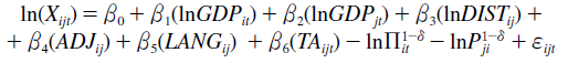 (1)
(1)Where ln denotes natural logarithms; Xijt is the value of the aggregate export flow from country i to country j in year t; GDPit (GDPjt) is gross domestic product, or GDP, in country i (j) in year t; DISTij is the bilateral distance between the economic centres of i and j; ADJij is a dummy variable assuming a value of one if the two countries share a common land border (and zero otherwise); LANGij is a dummy variable that takes a value of one if the two countries share a common language; TAijt is a variable indicating whether there is a TA between the two countries in year t, and lnP1–d (lnPji1–d) is exporter i’s (importer j’s) non-linear and unobservable MR term.
Baier and Bergstrand (2007) suggested estimating equation (1) by using bilateral (ij) fixed effects to account for variation in DIST, ADJ and LANG along with countrytime (it, jt) fixed effects to account for variation in GDPs and the MR. According to the theory this should generate an unbiased estimate of b6. They subsequently propose the use of panel techniques and estimation by fixed effects (FE) of the following equation:
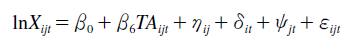 (2)
(2)Where hij is a country-pair fixed effect to capture all time-invariant bilateral factors influencing nominal trade flows; dit and }jt are exporter-time and importer-time fixed effects, respectively, to capture time-varying exporter and importer GDP, as well as all other time-varying country-specific effects that are unobservable in i and j and that influence trade, including the exporter’s and importer’s MR.
According to Anderson (2010), a major drawback to FE estimation in the gravity equation is its demolition of structure. As he puts it, «the econometrician blows up the building to get at the safe inside containing the inferred bilateral trade costs». In fact, introducing the three sets of dummies at country level (hij, dit and }jt) is not free of cost and it presents the shortcoming that it does not allow one to distinguish the effect of those determinants that are collinear with the introduced dummies, as is the case of the effect of distance, or the case of those variables included in the model which vary across countries (i or j) and time.
2.2 Estimation when using trade statistics at region-to-country level
Discontinuity in economic space does not just occur at the border but also within a country. Therefore, taking into account subnational variation might provide a more accurate assessment of the impact of a set of regressors on trade flows across countries, as large differences in country-level averages might be unrepresentative (Beugelsdijk and Mudambi, 2013). In a similar context to that of the present paper, Siroën and Yucer (2012) address the importance of dealing with within-country heterogeneity when analysing the impact of TAs, as the trade effects of TAs could be unevenly distributed across regions.
With regards papers that rely on the use of regional trade data, LeSage and Polasek (2008) use interregional trade data for Austria, while Llano-Verduras et al. (2011) use Spanish interregional trade data. Siroën and Yucer (2012) use trade among Brazilian states, Potters et al. (2014) and Thissen et al. (2013) use a unique dataset on bilateral trade between European NUTS2 regions. Nonetheless, interregional trade statistics are characterised by the fact that they are not publicly available. Another paper that uses regional trade statistics is Fratianni and Marchionne (2012), who use annual exports by Italian region and destination country. In that particular case, data are sourced from the Italian National Institute of Statistics and include all bilateral flows recorded by customs offices. Other examples include studies that use regional trade data for Japan, where international trade data are provided by the Japanese Customs of the Ministry of Finance at each international port (Hirose and Yoshida, 2012); for Poland (Ciżkowicz et al., 2013); and for Spain (Márquez-Ramos, 2016).
Given these recent advances in the availability of regional trade data, and although there is still a lack of information on region-to-region trade flows (see, for example, Gallego and Llano, 2014), we use information regarding trade flows from subnational geographical units to countries. We propose the use of regional trade statistics (region-to-country) as an alternative to country-to-country trade statistics in order to analyse the effect of specific regional integration processes on trade flows. We call this strategy «regionalising with regionalism». In this respect, it is worth highlighting that Thisse (2010) recommended examining the interaction between the regional and the international, stating that:
«The new fundamental ingredient that a multiregional setting brings about is that the accessibility to spatially dispersed markets varies across regions. [...] Any global change in this network such as market integration is likely to trigger complex effects [...] Accounting explicitly for a multiregional economy with different trade costs should rank high on the research agenda» (Page 293-294).
In this regard, related literature has already used subnational trade flows to analyse the so-called «border puzzle» (McCallum, 1995; Anderson and van Wincoop, 2003; Llano-Verduras et al., 2011; Behrens et al., 2012; Groizard et al., 2014; Gallego and Llano, 2014). However, there has been no previous attempt focusing on the effect of TAs on bilateral trade flows from specific regions in different countries to a sample of countries. We aim to fill this gap in the existing literature. In doing so, we apply our suggestion of «regionalising with regionalism», which stems from the recognition of the key role of subnational spatial variation.
3. The data
3.1 Sample
We use regional asymmetrical interaction data. That is, the observations are dyads, i.e. regional exports, and the importing partners are countries. Therefore, the number of origins is different from the number of destinations, and origins cannot be destinations. Asymmetrical interaction data has previously been used in a number of applications of the gravity equation to analyse the effect of RHS variables of interest at country level (for example, Jacks and Pendakur, 2010 and Florensa et al., 2015a). An advantage of using a region-to-country dataset is the decrease in the number of influential observations, or outliers, which usually characterise gravity studies at country-to-country level. A second advantage is that we avoid the selection bias that would arise from the correlation of the TA variable with differences in unobservables for partners with TAs versus partners without TAs, as we have subnational variation within a single country in one of the dimensions (i.e. origins).
We use an unbalanced panel for two Latin American countries (Argentina and Brazil) and two EU member states (Poland and Spain). These countries comprise a total of 86 exporting regions 3. We rely on a sample of 45 destination countries. The importing countries are: Algeria, Argentina *, Australia, Austria, Bangladesh, Belgium, Brazil *, Canada, Chile, China, Colombia, the Czech Republic, Denmark, Egypt, Finland, France, Germany, Greece, Hong Kong, India, Indonesia, Ireland, Italy, Japan, Jordan, Lebanon, Malaysia, Morocco, Mexico, the Netherlands, New Zealand, Pakistan, Poland *, Portugal, Singapore, South Africa, South Korea, Spain *, Sweden, Thailand, Tunisia, Turkey, the United Kingdom, the United States, Venezuela and Vietnam 4.
The choice of these 4 exporters (and the 45 destination countries) was made by searching two economic areas where integration strategies differ: Europe and Latin America. On the one hand, with regards European integration, the expansion of the EU was made possible through the accession of new member states, i.e. enlargement. In fact, the 13 CEECs that joined the EU under its Eastern enlargements had already signed TAs with the European Economic Community (EEC) prior to their inclusion 5. Ten of these countries joined the EU in May 2004, while Bulgaria and Romania joined in 2007 and Croatia in July 2013. It is important to highlight that once a country joins the EU, EU agreements automatically take effect, in accordance with the EC Treaty, the Treaty that established the European Community. For example, the 10 CEECs that joined the EU in 2004 became parties to the EEC’s free trade agreements and customs unions with third parties. In other words, once the 10 CEECs joined the EU in 2004, they became part of the European Common Market adopting the previously signed EU trade agreements. Consequently, all previous TAs between acceding countries and third parties terminated as of 1 May 2004 (European Commission, 2004).
On the other hand, in Latin America, Mercosur and CAN underwent a change in the integration level from a Preferential Trade Agreement (PTA) to a Free Trade Agreement (FTA) in 2005. Note that since 1980 these countries had been part of the Latin American Integration Association (LAIA), which established a PTA between 11 Latin American countries (Florensa et al., 2015a). However, different outcomes might have occurred for the two Latin American countries in this study. Firstly, we should recall that Brazil is a regional hegemon (Florensa et al., 2015a) and, secondly, that trade policy has undergone different changes in these countries. Also, it is worth mentioning that the modality of negotiating bloc-to-bloc (i.e. 4 countries in CAN + 4 countries in Mercosur) was replaced in 1999 by CAN negotiations with each Mercosur member (i.e. 4 + 1). As a result, in 1999 Colombia, Ecuador, Peru and Venezuela signed a TA with Brazil on tariff preferences as a first step towards the creation of an FTA between CAN and Mercosur. In 2000, CAN and Argentina signed a partial scope agreement of economic complementation, which took effect in August that year (Comunidad Andina, 2016). As Mercosur did not negotiate as a regional bloc, the trade preferences granted differ across Mercosur members. As a point in case, Florensa et al. (2015b) show the change in the effectively applied tariffs from 1994 to 2008 in Latin American countries. For example, while tariffs in Argentina for goods from LAIA fell by 77.32%, tariffs in Brazil fell by 83.39%.
Maintaining the focus on Latin American countries, Márquez-Ramos et al. (2015) demonstrate divergent effects of TAs on exports in different time periods; Latin America is characterised by economic instability and so results should not be generalised for extended periods 6. However, if we want to use regression analysis to understand the relationship between two variables, as is the case of TAs and trade flows, we need some sort of stability over time. Particularly in the case of developing and transition countries, we suggest analysing the effect of TAs on trade flows using «regionalised» data over stable periods. Therefore, we focus on the period 2000-2008. Additionally, this time period covers the years immediately after the convergence criteria were first met for the European and Monetary Union and covers the accession of 10 CEECs to the EU in 2004 as well as Bulgaria and Romania in 2007 7.
3.2 Variables
We determine the existing TAs that involve the two EU member states and those involving the two Mercosur members during the period 2000-2008. To do so, we use the database on Economic Integration Agreements8 available from the Bergstrand’ webpage (http://www3.nd.edu/~jbergstr). We then construct a TA binary variable to explore the evolution of national exports and the existence (or non-existence) of TAs.
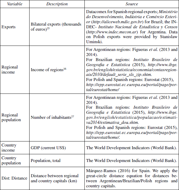
Next, we establish a set of RHS variables for the exporting regions in the four countries considered in this paper as well as for trading partners over the time period 2000-2008. In line with previous literature, we include exporter’s and importer’s income, relative factor endowments, geographical distance, and a binary variable for TA. To calculate the geographical distance between regional capitals and country capitals, we used data provided by Márquez-Ramos (2016) for Spain, and applied the great-circle distance equation for distances between Argentinean/Brazilian/Polish9 regions and the capital of each corresponding importing country10. With regards to regional-level population and income data, GDP and population for Polish and Spanish regions were obtained from Eurostat. For Brazilian regions, GDP was obtained from the Regional Accounts for Brazil at the Instituto Brasileiro de Geografia e Estatística, and population estimates for the Brazilian municipalities were used to construct the data on population at the regional level. Finally, Argentinean regional population and income data is taken from Figueras et al. (2013 and 2014)11. Table A.1 in Appendix A lists the variables and data sources used.
3.3 Descriptive analysis
Before proceeding to the econometric analysis, we will briefly analyse the data. First, we illustrate graphically the importance of the variation in export data from different regions within a country. Figures B1,B2,B3,B4 in Appendix B display the average (log of) exports (in thousands of euros) to importers in 2008 by region at NUTS2 level, while Figures B5,B6,B7,B8 display data for 2000. These maps use a dark colour to show the regions where the most important international trade flows were concentrated in 2008 and 2000 (darker colours represent higher flow levels while lighter colours represent lower flow levels). This preliminary descriptive analysis provides evidence about with-in-country variability of exports. We compare the figures of export flows in 2000 and 2008 and it seems that the most important economic centres are the same in both 2000 and 2008. Overall, exports increased from 2000 to 2008, although we observe smaller increases (or even a reduction) in relatively small north-eastern regions in Brazil, such as Paraíba and Rio Grande do Norte, and in Polish regions neighbouring the Ukraine and Belarus, i.e. Lubelskie, Podkarpackie and Podlaskie 12, Argentinean and Spanish regional exports seem to have grown at a lower rate than in Brazil and Poland; in Spain, however, this rate is more balanced among regions. In Argentina, exporting centres are concentrated in regions neighbouring Buenos Aires, such as Córdoba, Entre Ríos and Santa Fé, with a few exceptions, such as Chubut, Mendoza and Salta.
Secondly, Figures C1,C2,C3,C4 in Appendix C give a sense of correlations and show the evolution of average exports by country when a TA exists, and when it does not. The black solid line shows the evolution of the average exports with trading partners where TAs exist, whereas the dashed line shows the evolution of the average exports when there are no TAs with trading partners. The trends in the figures show that exports are higher when they are destined for trading partners with TAs. This is the case for both European and Latin American countries, although the difference is more pronounced in the case of the EU, particularly for Spain (Figure C.4). This said, although Brazil (Figure C.2) shows that exports to trading partners both with and without TAs increased over the time period under study, a more pronounced positive trend is observed for the no-TA group of countries from 2003 onwards, narrowing the existing gap. As for Poland, Figure C.3 clearly shows the change on joining the EU in 2004, as all TAs between Poland and third parties terminated on 1 May 2004. For example, Poland had a Non-Reciprocal Preferential Trade Agreement with the US, however, Poland’s USGSP status terminated when it joined the EU. Therefore, the immediate positive effect of new TAs might not be enough to compensate for the negative effects of terminating prior TAs, as trade costs increased with a number of third countries that did not have TAs with the EU-15. With regards Argentina, Figure C.1 indicates that the average regional exports to the sample of destination countries under study was lower in 2008 than in 2000. Conclusions here should be taken with care for two main reasons. Firstly, taking the average of the logarithm of exports might actually be distorting the participation of the largest provinces and, secondly, the variation over time observed in Argentinean regions has led to lower average exports from a number of peripheral regions (Appendix B) 13. Interestingly, this trend suggests that trade integration may exacerbate agglomeration forces in the largest economic centres in a number of countries, as is the case with Argentina, indicating that it might be more appropriate to take into account regional variability (within country) in gravity-type models. It is also worth highlighting that disparities in the consequences of economic integration within countries are a greater cause for concern than disparities between countries. As a matter of fact, regional differences between the citizens of the same country are much less socially excusable, economically justifiable or politically acceptable (Figueras et al., 2013 and 2014).
Finally, in order to show how «open» regions are, Appendix D shows the maps with the (logarithm of) exports per capita in 2008 by region (darker grey colours indicate higher exports per capita). According to the export-to-population ratio, the most «open» regions in Argentina (Map D.1) are Santa Fé, Córdoba, Tierra del Fuego, Chubut and Buenos Aires; in Brazil (Map D.2) the most «open» regions are located in south-eastern and central-western Brazil. In Poland (Map D.3), Mazowieckie (where the capital is located) is the most «open» region in 2008, followed by Slaskie, Dolnoslaskie and Wielkopolskie. The eastern regions in Poland clearly have the lowest exports per capita within this country. Finally, regions located in the north-east of Spain, such as Catalonia, Navarre and the Basque Country, register the highest exports per capita in Spain.
4. On the effect of the EU’s CEEC enlargement and the CAN- Mercosur agreement
4.1 Methodological issues
As mentioned above, we exploit subnational spatial variation in the challenging analysis facing international trade researchers into the effect of regional integration on international trade flows 14. Specifically, we analyse the effect of two exogenous changes in the regional integration status on exports arising from subnational regions. To do so, we assume that both the EU’s CEEC enlargement and the entry into force of the CAN- Mercosur agreement are exogenous when the dependent variable is exports of subnational units in a gravity equation, as these agreements have been negotiated at country-level.
For the case of EU countries over the period 2000-2008, the model that we consider is:
 (3)
(3)Where ln denotes natural logarithms, Xijt denotes exports from (Spanish or Polish) region j to country t in year t, Y is the product of GDP for exporter i and importer j, the variable RLF is defined as the absolute value of the difference between trading partners’ per capita GDP and measures the difference in terms of relative factor endowments (see Serlenga and Shin, 2007), and Dist denotes distance. TAjt is a binary indicator that equals one if the importing trading partner had the status of Common Market in year t.
It is worth mentioning that there are two possible motivations for this kind of agreement: to ease the international trade relations between two consolidated partners; or to open a new channel of international trade and start to exploit the gains to be had from trade openness. Although the second motivation is exogenous, the first is more problematic. Therefore, we include bilateral fixed effects, which are perfectly collinear with the distance variable, as well as time fixed effects to avoid endogeneity 15:
 (4)
(4)where hij are the exporter-importer fixed effects, which contains factors that are constant over time, and it are the time fixed effects. We are interested in the average exports before and after the change of the integration status between the exporter and the importer, so we transform equation (4) as follows:
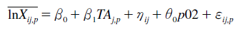
 (5)
(5)Where p denotes the period before the exogenous change in May 2004 (p01 = 2000-2003) and after (p02 = 2005-2008), and p02 is a dummy variable for the second period. Note that averaging income and the variable RLF over the four years before and after 2004 considerably simplifies equation (5) as variability that would be captured by these magnitudes can be included in the bilateral fixed effects in the region-to-country gravity approach used in this paper. To justify this approach, we highlight the fact that those regions that, on average, had comparable «mass» before 2004 also had comparable «mass» after 2004. As a matter of fact, no relevant structural changes have occurred over the nine-year time period taken into account with regards income and income per capita (required to construct RLF). Then, we have:
 (6)
(6)Finally, differencing removes unobserved heterogeneity:
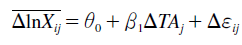 (7)
(7)Therefore, we regress the change of the log of (average) regional bilateral exports on the change in the TA variable for the case of the EU exporters 16. The exercise is identical for the CAN-Mercosur integration in 2005 for Argentina and Brazil, although in that case the periods before and after the change are 2000-2004 and 2005- 2008, respectively 17.
4.2 Main results
The results of estimating the first-differenced equation (7) by Ordinary Least Squares (OLS) appear in Table 1. According to these results, average exports are significantly higher in the most recent period (i.e. 2005-2008) than in the pre-2005 period in the four countries under study. The EU enlargement did not have a significant effect on regional exports from Poland, although it did have a positive and significant effect on Spanish regional exports. Specifically, the EU enlargement increased average Spanish regional export flows by about 46% [exp(0.376) - 1 = 0.4564]. With regard to the CAN-Mercosur TA, we find that it increased average exports from Brazilian regions by 102%; however, results show that the change in the integration status with CAN members had a non-significant effect for Argentinean regional exports. Nonetheless, it is worth noting that results do not indicate that the effect of deeper integration is generally higher for Brazil than for Argentina, but rather that this specific change, i.e. the change of integration status from a PTA to an FTA with the two affected importer countries (in our sample Colombia and Venezuela), was positive and significant for Brazil. It might therefore be expected that exports have grown to a larger extent in Brazil than in Argentina as a consequence of CAN-Mercosur integration, as Florensa et al. (2015b) showed Brazil was better able to reduce tariff rates with other Latin American countries.
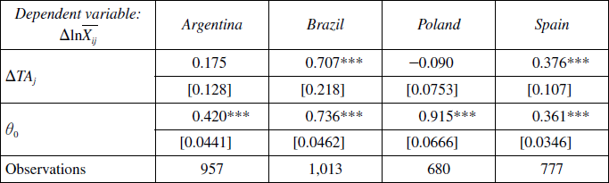
Notes: *** indicates significance at 1 per cent level. Robust standard errors are provided in square brackets. OLS estimator.
Notes: *** indicates significance at 1 per cent level. Robust standard errors are provided in square brackets. OLS estimator.
5. Robustness and benchmarking
In Argentina, there was a devaluation of the peso from 1ARS = 1USD to 3.36ARS = 1USD in January 2002. In addition, the inflation rate for 2002 was 40.9%. After the bank runs of 2001 and one of the defaults, Argentina was faced with economic and political disorder throughout 2002 (Thomas and Cachanosky, 2015). In this section, we therefore first perform an initial robustness check by running the same analysis for Argentina, but removing years 2000 and 2001. The result is remarkably similar, with a coefficient of 0.178 and a standard error of 0.127. In other words, we see a non-significant effect of the change of the integration status from a PTA to an FTA at the usual levels of statistical significance.
Secondly, compared to earlier research on exports from Polish regions, a number of changes were found: 1) the inflow of FDI has contributed to increased export dynamics of some regions, with values higher than the average for Poland; 2) the share of Mazowieckie (capital region) was seen to be decreasing; 3) other CEECs, such as the Czech Republic, have registered a relative rise in overall Polish exports. This is the case for southern regions of Poland. Finally, western and southern regions of Poland benefited greatly in terms of intensified foreign trade links (Gawlikowska-Hueckel and Uminski, 2013; Uminski, 2014). The fact that our findings show that Poland, a transition economy, did not register a significant positive effect on trade flows for regions over the period under review, may be a result of the fact that the aforementioned research examined Poland’s regional export changes from a Polish perspective (Gawlikowska-Hueckel and Uminski, 2013; Uminski, 2014). But generally speaking, this paper takes a wider view of the four countries under study. One explanation for our findings could be that most foreign-trade structural changes in Poland occurred when Poland signed the FTA agreement with the EU for industrial products in the 90s. Therefore, any changes in trade that took place after Poland’s entry into the EU were primarily those relating to other CEECs that joined the EU at the same time as Poland. Paradoxically then, it appears that the changes occurred in relation to non-EU countries 18. To check this hypothesis, we re-run the analysis for Poland including only the Czech Republic (the only new EU country in our sample of destination countries) as the trading partner that experienced a change in the integration status. Then, we estimate equation (7), but this time only for Malopolskie, Mazowieckie, Opolskie, Podlaskie, Slaskie and Swietokrzyskie as exporters, as they are the regions in Poland where export intensity is high between entities established in particular regions and the new EU (Gawlikowska-Hueckel and Umiński, 2013). Our results validate this hypothesis: the export flows from the Polish regions with high-intensity export relations with new EU countries increased by about 36% [exp(0.306) - 1 = 0.3579] as a consequence of the EU enlargement 19.
As a benchmark, we take into account year variability and we use panel techniques to analyse the effect of TAs by estimating equation (4). It is worth mentioning that by doing so, the number of observations increases considerably, although we are unable to isolate the effect of the EU enlargement in May 2004, or the effect with the CAN-Mercosur agreement.
To analyse whether regions in the four countries export more after the exogenous changes in economic integration, we consider the variable TA_new that interacts the traditionally included binary TA variable 20 with two additional dummies: one, with a value of one after 2004, the other with a value of one for importing countries changing their regional integration status.
Panel data allows researchers to control for unobservable bilateral fixed effects (see subsection 2.1 of the present paper). The random effects (RE) estimator requires there to be no correlation between the covariates and the (dyadic) unit effects. Since the RE model does not estimate separate unit effects, any correlation between the explanatory variables and unobserved heterogeneity can imply an omitted variable that produces bias in the estimates of the parameters. Then, the RE estimator yields consistent estimates only when the regressors are uncorrelated with the unobservable dyadic fixed effect. However, it is likely to find correlation among some RHS variables and the unobservable bilateral individual effects (i.e. there is endogeneity). This correlation can be verified with the Hausman test. Although FE is a straightforward way to tackle such a problem and gives unbiased estimates of time-varying variables, it impedes the analysis of time-invariant variables.
According to Clark and Linzer (2015), the most common objection to the use of RE - the violation of the «critical» modelling assumption that the regressor and the unit effects are uncorrelated —turns out to be an insufficient justification for choosing fixed rather than random effects. In fact, the Hausman test is primarily intended to analyse whether the coefficients obtained in the two methods differ significantly. As Clark and Linzer (2015) point out: «The presence of non-zero correlation between the independent variable and unit effects is neither a sufficient nor a necessary condition for choosing a fixed-effects model» (Clark and Linzer, 2015, p. 406). As a consequence, we provide the results from both FE and RE.
Finally, in line with Egger (2002), Carrère (2006), Serlenga and Shin (2007), Mitze (2012) and Gallego and Llano (2014) we rely on Hausman and Taylor (1981) (or HT) to estimate equation (4)21. The HT estimator is based on an instrumental variable estimator which uses both the between and within variation of the strictly exogenous variables as instruments. In this approach, we follow Carrère (2006) and Gallego and Llano (2014) in considering GDP as a source of endogeneity.
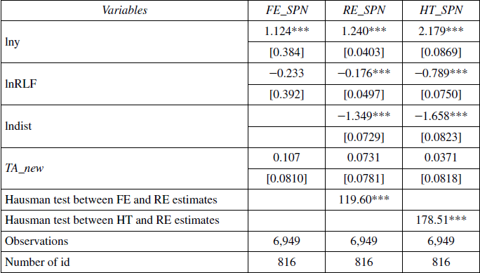
Tables 2, 3, 4 and 5 show the results by FE, RE and HT for Argentina, Brazil, Poland and Spain, respectively. We find that the effect of income on trade intensity is positive and significant, while the effect of distance is negative and significant in all cases, with the exception of income in the FE regression for Argentina, which is not statistically significant. The impact of the differences in factor endowments (RLF) is negative and significant in the estimation by RE and HT for Argentina, Brazil and Spain. For Poland, increasing differences in factor endowments result on higher intensity of exports, according to the RE estimation. This variable loses significance when using the FE estimator, and its associated estimated coefficient reverses sign in the case of Argentina.
With regards our variable of interest, the estimated coefficient for TA_new is found to be positive and significant only in the case of Brazil and we fail to support the previous evidence found for Spain. The international financial crisis that severely affected Europe might be behind these results when taking into account yearly data. Although the results illustrate the difficulty in isolating the effect of the two regional integration processes taken into account, they support the empirical evidence obtained in the main analysis for Argentina, Brazil and Poland.
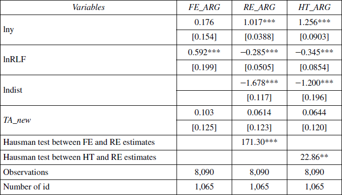
Standard errors in square brackets.
*** p < 0.01, ** p < 0.05, * p < 0.1
FE denotes fixed effects, RE denotes random effects and HT denotes the Hausman-Taylor estimator. In HT the likely endogenous variable is the product of GDPs. Year dummies are omitted to save space. Time period: 2000-2008.
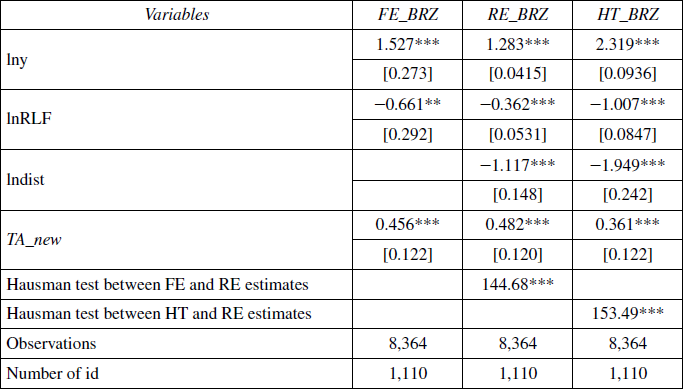
Standard errors in square brackets.
*** p < 0.01, ** p < 0.05, * p < 0.1.
FE denotes fixed effects, RE denotes random effects and HT denotes the Hausman-Taylor estimator. In HT the likely endogenous variable is the product of GDPs. Year dummies are omitted to save space. Time period: 2000-2008.
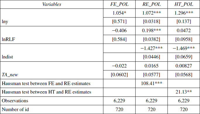
Standard errors in square brackets.
*** p < 0.01, ** p < 0.05, * p < 0.1.
FE denotes fixed effects, RE denotes random effects and denotes the HT Hausman-Taylor estimator. In HT the likely endogenous variable is the product of GDPs. Year dummies are omitted to save space. Time period: 2000-2008.
Standard errors in square brackets.
*** p < 0.01, ** p < 0.05, * p < 0.1..
FE denotes fixed effects, RE denotes random effects and denotes the HT Hausman-Taylor estimator. In HT the likely endogenous variable is the product of GDP’s. Year dummies are omitted to save space. Time period: 2000-2008.
6. The four-country tale
The results obtained raise the following questions 22:
-
1) Why have Argentinean regions not benefited from the CAN-Mercosur agreement?
2) Why have Brazilian regions benefited from the CAN-Mercosur agreement?
3) Why have only a few regions in Poland benefited from the EU enlargement?
4) Why have Spanish regions benefited from the EU enlargement?
A possible explanation is that trade integration leads to countries as a whole becoming more specialized, but the consequences will naturally be different in the various countries in question. In Europe, established EU members (such as Spain), i.e. where the specialization process has long been underway, might have increased their market potential with the EU enlargement. Conversely, for the new transition countries (such as Poland) the change on joining the EU and the end of TAs with third parties might have had an impact on comparative advantages at regional level. In Latin America, both Argentina and Brazil suffer from strong regional inequalities. Additionally, there are important divergences in their economic integration strategies that might go some way to explaining the results obtained. On the one hand, Argentina has implemented economic policies that might have distorted regional trade patterns and a consequence may have been that Argentinean regions did not benefit from the CAN-Mercosur agreement 23. On the other hand, the strategic view that Brazil has taken of regional integration as a means of enhancing its power and influence in international fora as well as in Latin America (Doctor, 2007) is consistent with the obtained results.
7. Conclusion and discussion
We have used trade data at finer levels of geographical disaggregation than country-level to analyse the effect of two regionalism experiences, which we view as two exogenous examples of regional integration in a gravity approach. Then, we contribute to the literature by analysing the effect of extending trade preferences within two existing TAs in Latin America, i.e. Mercosur and the Andean Community, and the EU’s CEEC enlargement.
Using region-to-country trade data is rare as few countries readily make such data publicly available. Recent examples that use regional trade data include studies of Spain (Márquez-Ramos, 2016), Japan (Hirose and Yoshida, 2012) and Poland (Ciżkowicz et al., 2013; Gawlikowska-Hueckel and Uminski, 2013; Uminski, 2014). So although this methodology allows us to rule out possible endogeneity bias in RHS variables at country level 24, there is a long way to go until international trade economists are able to base international trade analysis on regional trade statistics. Interestingly, Courant and Deardorff (1992) proved that the disparities across regions within countries can cause international trade. In fact, the conclusions formulated at the country level ignore a whole range of regional variations (Gawlikowska-Hueckel and Uminski, 2013).
We found an unbiased partial effect of EU enlargement in May 2004 and the CAN-Mercosur TA on regional exports from Argentina, Brazil, Poland and Spain. Our results provide evidence that Brazil has benefited from extending trade preferences to members of another existing Latin American TA (i.e. CAN) in terms of regional exports. We also find that the EU’s CEEC enlargement had a significant positive effect on regional exports from Spain. Conversely, a non-significant effect of the EU enlargement and the CAN-Mercosur TA was found for Poland and Argentina, respectively, over the time period under study. These results have been validated in a panel data benchmark, using fixed effects, random effects and a Hausman-Taylor approach. Nonetheless, we failed to find evidence of a positive and significant effect of the change in the integration status of new transition EU countries for Spain.
Although Poland, a transition economy, is involved in a process of deep integration, i.e. the EU, our results show that recent regionalism has not had a significant positive effect on trade flows from Polish regions over the time period considered, as seen not only in the main analysis, but also in the robustness analysis. However, the export flows from the Polish regions with high-intensity export relations with new EU countries increased as a consequence with the EU enlargement.
Acknowledgments
The author gratefully acknowledges the support and collaboration of Universitat Jaume I and Generalitat Valenciana (P1-1B2013-06; PROMETEOII/2014/053). Thanks to Àlvar Franch Doñate for his contribution to database processing. I would also like to thank Benedikt Heid, María Luisa Recalde and Stanislaw Uminski for their very helpful comments and suggestions.
References
Anderson, J. E. (2010): «The gravity model», National Bureau of Economic Research (No. w16576).
Anderson, J. E., and van Wincoop, E. (2003): «Gravity with Gravitas: A Solution to the Border Puzzle», American Economic Review, 93(1).
Baier, S. L., and Bergstrand, J. H. (2007): «Do Free Trade Agreements Actually Increase Members’ International Trade?», Journal of International Economics, 71, 1, 72-95.
Baier, S. L., Bergstrand, J. H. and Feng, M. (2014): «Economic integration agreements and the margins of international trade», Journal of International Economics, 93(2), 339-350.
Baier, S. L., Bergstrand, J. H., and Vidal, E. (2007): «Free trade agreements in the Americas: Are the trade effects larger than anticipated?», The World Economy, 30(9), 1347-1377.
Baldwin, R., and Taglioni, D. (2006): «Gravity for Dummies and Dummies for Gravity Equations», NBER Working Papers, 12516, National Bureau of Economic Research, Inc.
Behrens, K., Ertur, C., and Koch, W. (2012): «“Dual” gravity: Using spatial econometrics to control for multilateral resistance», Journal of Applied Econometrics, 27(5), 773-794.
Bergstrand, J. H. (1985): «The gravity equation in international trade: Some micro-economic foundations and empirical evidence», The Review of Economics and Statistics, 67(3), 474-481.
Bergstrand, J. H. (1989): «The generalized gravity equation, monopolistic competition, and the factor-proportions theory in international trade», The Review of Economics and Statistics, 71(1), 143-153.
Beugelsdijk, S., and Mudambi, R. (2013): «MNEs as border-crossing multi-location enterprises: The role of discontinuities in geographic space», Journal of International Business Studies, 44(5), 413-426.
Carrère, C. (2006): «Revisiting the effects of regional trade agreements on trade flows with proper specification of the gravity model», European Economic Review, 50(2), 223-247.
Ciżkowicz, P., Rzońca, A., and Uminski, S. (2013): «The determinants of regional exports in Poland —a panel data analysis», Post-Communist Economies, 25(2), 206-224.
Clark, T. S., and Linzer, D. A. (2015): «Should I use fixed or random effects?», Political Science Research and Methods, 3(2), 399-408.
Comunidad Andina (2016): Relaciones Externas. Mercosur. Available at http://www.comunidadandina.org (retrieved June 24, 2016).
Courant, P. N., and Deardorff, A. F. (1992): «International Trade with Lumpy Countries», Journal of Political Economy, 100(1), 198-210.
Damill, M., and Frenkel, R. (2013): «La economía argentina bajo los Kirchner: una historia de dos lustros», Documentos Técnicos, Iniciativa para la Transparencia Financiera.
Doctor, M. (2007): «Why Bother with Inter-Regionalism? Negotiations for a European Union- Mercosur Agreement», Journal of Common Market Studies, 45(2), 281-314.
Egger, P. (2002): «An econometric view on the estimation of gravity models and the calculation of trade potentials», The World Economy, 25(2), 297-312.
European Commission (2004): Termination of trade agreements due to enlargement. Notification from the European Communities and its member states to the committee on regional trade agreements. Directorate-General for Trade, Brussels, 20 September 2004.
Figueras, A. J., Cristina, A. D., Blanco, V., and Capello, M. L. (2013): «Estudio sobre la convergencia regional: las nuevas evidencias del siglo xxi», Paper presented at 46 Jornadas Internacionales de Finanzas Públicas, Córdoba, Argentina, Universidad Nacional de Córdoba, Facultad de Ciencias Económicas, September.
Figueras, A. J., Cristina, A. D., Blanco, V., Iturralde, I., and Capello, M. L. (2014): «Un aporte al debate sobre la convergencia en Argentina: la importancia de los cambios estructurales», Revista Finanzas y Política Económica, 6(2), 287-316, http://dx.doi.org/10.14718/revfinanzpolitecon.2014.6.2.4.
Florensa, L. M., Márquez-Ramos, L., and Recalde, M. L. (2015a): «The effect of economic integration and institutional quality of trade agreements on trade margins: evidence for Latin America», Review of World Economics, 151(2), 329-351.
Florensa, L. M., Márquez-Ramos, L., Martínez-Zarzoso, I., and Recalde, M. L. (2015b): «Regional versus global production networks: where does Latin America stand?», Applied Economics, 47(37), 3938-3956.
Fratianni, M., and Marchionne, F. (2012): «Trade costs and economic development», Economic Geography, 88(2), 137-163.
Gallego, N., and Llano, C. (2014): «The Border Effect and the Nonlinear Relationship between Trade and Distance», Review of International Economics, 22(5), 1016-1048.
Gawlikowska-Hueckel, K., and Uminski, S. (2013): «Competitiveness at the regional level: export-oriented approach for Poland», in Jóźwik, B., and Stępniewski, T. (ed.), Central and Eastern Europe: convergence, integration and security. Yearbook of the Institute of East-Central Europe, vol. 11, Issue 6, 131-156.
Groizard, J. L., Marques, H., and Santana, M. (2014): «Islands in Trade: Disentangling Distance from Border Effects», Economics: The Open-Access, Open-Assessment E-Journal, 8 (2014-40): 1-46.
Hausman, J. A., and Taylor, W. E. (1981): «Panel data and unobservable individual effects», Econometrica, 49(6), 1377-1398.
Head, K., and Mayer, T. (2014): «Gravity equations: Workhorse, toolkit, and cookbook», in Handbook on International Economics, vol. 4, Elsevier-North-Holland, 131-195.
Hirose, K., and Yoshida, Y. (2012): «Intra-National Regional Heterogeneity in International Trade: Foreign Growth on Exports and Production of Domestic Regions», Discussion Papers, 54, Kyushu Sangyo University, Faculty of Economics.
Jacks, D. S., and Pendakur, K. (2010): «Global Trade and the Maritime Transport Revolution», Review of Economics and Statistics, 92(4): 745-755.
LeSage, J. P., and Polasek, W. (2008): «Incorporating transportation network structure in spatial econometric models of commodity flows», Spatial Economic Analysis, 3 (2), 225-245.
Llano-Verduras, C., Minondo, A., and Requena-Silvente, F. (2011): «Is the Border Effect an Artefact of Geographical Aggregation?», The World Economy, 34(10), 1771-1787.
Márquez-Ramos, L. (2016): «Port facilities, regional spillovers and exports: Empirical evidence from Spain», Papers in Regional Science, 95(2), 329-351.
Márquez-Ramos, L., Florensa, L. M., and Recalde, M. L. (2015): «Economic Integration Effects on Trade Margins: Sectoral Evidence from Latin America», Journal of Economic Integration, 30 (2), 269-299.
Márquez-Ramos L, and Martínez-Zarzoso, I. (2014): «Trade in intermediate goods and Euro- Med production networks», Middle East Development Journal, 6(2), 215-231.
McCallum, J. (1995): «National Borders Matter: Canada-U.S. Regional Trade Patterns», American Economic Review, 85(3), 615-623.
Mitze, T. (2012): Empirical Modelling in Regional Science: Towards a Global Time-Space- Structural Analysis (vol. 657), Springer Science & Business Media.
Potters, L., Conte, A., Kancs D’A., and Thissen M., (2014): «Data Needs for Regional Modelling: A Description of the Data used in Support of RHOMOLO», Publications Office of the European Union.
Serlenga, L., and Shin, Y. (2007): «Gravity models of intra-EU trade: application of the CCEPHT estimation in heterogeneous panels with unobserved common time-specific factors», Journal of Applied Econometrics, 22(2), 361-381.
Siroën, J. M., and Yucer, A. (2012): «The impact of MERCOSUR on trade of Brazilian states», Review of World Economics, 148(3), 553-582.
Soete, S., and Van Hove, J. (2015): «Dissecting the trade effects of Europe’s economic integration agreements», Available at SSRN 2587666.
Thisse, J. F. (2010): «Toward a unified theory of economic geography and urban economics», Journal of Regional Science, 50(1), 281-296.
Thissen, M., Diodato, D., and van Oort, F. G. (2013): «Integration and Convergence in Regional Europe: European Regional Trade Flows from 2000 to 2010», PBL Netherlands Environmental Assessment Agency.
Thomas, C., and Cachanosky, N. (2015): «Argentina’s Post 2001 Economy and the 2014 Default», Department of Economic. Metropolitan State University of Denver. Available at SSRN.
Uminski, S. (2014): «Integration of Poland’s regions with the European Union-Assessment of intra industry trade relations», European Integration Studies, 8, 93-98.
Appendix A
25 Data on Argentinean and Brazilian exports were originally obtained in US Dollars, so they have been converted to Euros using the European Central Bank (ECB) reference exchange rate, (annual 2000- 2008) US dollar/euro.
26 To compute the GDP in Brazilian regions, we use aggregate national figures about the composition of GDP (in R$ 1.000.000) in combination with data on the share of GDP by Brazilian region.
27 With regards to population in Brazilian regions, there are no data available for the year 2000 so we use the average from 1999 and 2001. Due to data availability, we also estimate the population in Brazilian regions in 2007 and 2008 as follows: first, by constructing the rate of the increase in population from 2002 to 2006, and second, by using the calculated average growth rate of population by region to estimate the number of inhabitants in 2007 and 2008.
Appendix B
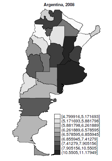
Figure B.1
Average Argentinean exports in 2008, by region
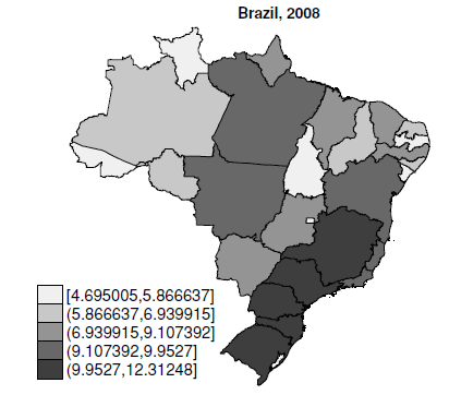
Figure B.2
Average Brazilian exports in 2008, by region
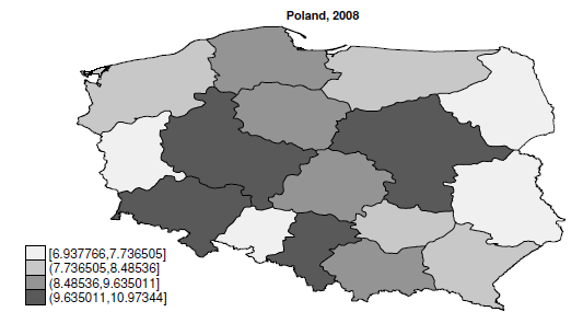
Figure B.3
Average Polish exports in 2008, by region
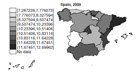
Figure B.4
Average Spanish exports in 2008, by region
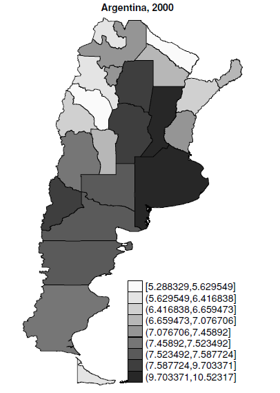
Figure B.5
Average Argentinean exports in 2000, by region
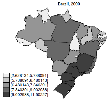
Figure B.6
Average Brazilian exports in 2000, by region
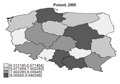
Figure B.7
Average Polish exports in 2000, by region
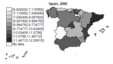
Figure B.8
Average Spanish exports in 2008, by region
Appendix C
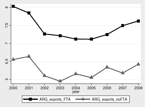
Figure C.1
Average exports from Argentinean regions (in logs)
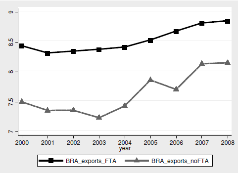
Figure C.2
Average exports from Brazilian regions (in logs)
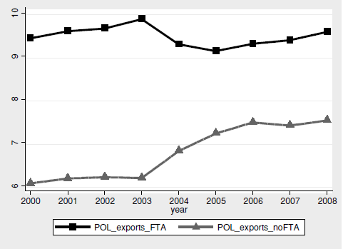
Figure C.3
Average exports from Polish regions (in logs)
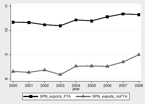
Figure C.4
Average exports from Spanish regions (in logs)
Appendix D
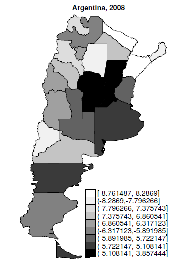
Figure D.1
Average Argentinean exports per capita in 2008, by region
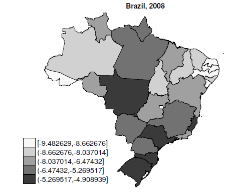
Figure D.2
Average Brazilian exports per capita in 2008, by region
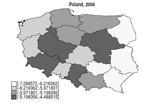
Figure D.3
Average Polish exports per capita in 2008, by region
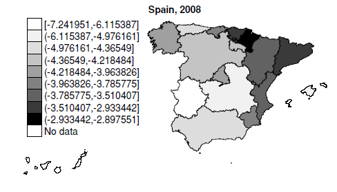
Figure D.4
Average Spanish exports per capita in 2008, by region
Notes
Author notes
undefined
Additional information
JEL Classification: F14; F15; R10
Clasificación JEL: F14; F15; R10