European Regional Policy
The 2019 assessment of the macroeconomic effects of the European Fund for Strategic Investments with the RHOMOLO-EIB model
Evaluación de 2019 de los efectos macroeconómicos del Fondo Europeo para Inversiones Estratégicas con el modelo RHOMOLO-EIB
The 2019 assessment of the macroeconomic effects of the European Fund for Strategic Investments with the RHOMOLO-EIB model
Investigaciones Regionales - Journal of Regional Research, no. 45, pp. 5-15, 2019
Asociación Española de Ciencia Regional

This work is licensed under Creative Commons Attribution-NonCommercial 4.0 International.
Received: 11 December 2019
Accepted: 16 December 2019
Abstract: The European Fund for Strategic Investments (EFSI) is the financial pillar of the Investment Plan for Europe. It tackles the post-crisis investment gap in the European Union (EU) and aims to revive investment in key areas in all the EU Member States. EFSI was launched in 2015 jointly by the European Investment Bank (EIB) Group and the European Commission. Every year, macroeconomic impact assessments are carried out using the spatial dynamic RHOMOLO-EIB model in order to gauge jobs and growth impact of the EFSI-supported operations in the EU. This article illustrates the methodology used for the assessment and reports the result of the latest set of simulations, corresponding to the portfolio of all approved EFSI-supported operations as of the June 13th EIB Board of Directors meeting, 2019. According to the results, EFSI is contributing significantly to job creation and growth. The estimates suggest that, by 2019, more than 1 million jobs are expected to be created thanks to the approved operations (1.7 million by 2022), with a positive contribution to GDP of 0.9% (1.8% expected by 2022) over the baseline.
Keywords: Spatial general equilibrium, fiscal policy, investment.
Resumen: El Fondo Europeo para Inversiones Estratégicas (FEIE) es el pilar financiero del Plan de Inversiones para Europa. Aborda la brecha de inversión posterior a la crisis en la Unión Europea (UE) y tiene como objetivo revivir la inversión en áreas clave en todos los Estados miembros de la UE. El FEIE se lanzó en 2015 conjuntamente por el Banco Europeo de Inversiones (BEI) y la Comisión Europea. Cada año, las evaluaciones de impacto macroeconómico se llevan a cabo utilizando el modelo espacial dinámico RHOMOLO-EIB para medir el empleo y el impacto de las operaciones respaldadas por el FEIE en la UE. Este artículo ilustra la metodología utilizada para la evaluación e informa el resultado del último conjunto de simulaciones, correspondiente a la cartera de todas las operaciones aprobadas respaldadas por el FEIE a partir de la reunión de la Junta Directiva del BEI del 13 de junio de 2019. Según los resultados, FEIE está contribuyendo significativamente a la creación de empleo y al crecimiento. Las estimaciones sugieren que, para 2019, se espera que se hayan creado más de 1 millón de empleos gracias a las operaciones aprobadas (1,7 millones para 2022), con una contribución positiva al PIB del 0,9% (1,8% esperado para 2022) respecto al escenario base.
Palabras clave: Equilibrio general espacial, política fiscal, inversión.
1. Introduction
In 2014, the European Union (EU) was still facing the consequences of the 2008 economic and financial crisis. This led the European Commission and the European Investment Bank (EIB) to launch the Investment Plan for Europe, also known as the Juncker Plan (EU, 2015). It has three complementary pillars: The first pillar, the European Fund for Strategic Investments (EFSI), implemented by the EIB Group, aims to mobilise finance for investments. The second pillar is dedicated to support investment in the real economy, by improving the pipeline of investable projects and by strengthening the provision of advisory services to project promoters. The European Investments Advisory Hub and the European Investment Project Portal have been established to help investment finance reach the real economy. The third pillar focuses on enabling an investment friendly environment in Europe by removing barriers to investment both nationally and at EU level. The first pillar, EFSI, was set-up with the aim to mobilise at least €315 billion of investment in the EU by mid-2018. The key to fulfilling this objective was a €16 billion guarantee from the EU and €5 billion contribution from the EIB Group in support of EFSI. In December 2017, the European Council and the Parliament extended the duration of EFSI by two years, dubbed as EFSI 2.0, and increased its investment target to at least €500 billion by 2020 (EU, 2017). To this end, the EU Guarantee was also increased to €26 billion, and the EIB Group nominal contribution increased to no less than €7.5 billion.
EFSI supports strategic investments in key areas of European interest. The eligible sectors include the following: smaller companies, RDI, transport, energy, environment and resource efficiency, digital, and social infrastructure. EFSI 2.0 introduced two additional new sectors: bioeconomy and regional development. EFSI 2.0 also brought an enhanced focus on sustainable investments in all sectors to contribute to meeting COP21 targets and to help deliver on the transition to a resource efficient, circular and low-carbon economy (Rogelj et al., 2016). While being dependant of the demand-driven nature of EFSI, EFSI 2.0 set a new 40% target for EFSI financing under the Infrastructure and Innovation Window implemented by the EIB (excluding EFSI financing to SMEs and small Mid-Caps) in relation to project components that contribute to climate action. The implementation of EFSI and in particular the compliance with the objectives set in the EFSI Regulation are reported on an annual basis to the European Parliament and to the Council. These EIB Group Reports are public and accessible on the EFSI Steering Board page of the EIB website.1 In addition, there is a regular assessment of the overall macroeconomic impact of EFSI operations. That is because, in addition to the direct impact of investments, these operations produce both indirect and induced effects in the economy.
Regular macroeconomic impact assessment of EFSI is carried out jointly by the EIB and the European Commission's Joint Research Centre (JRC), and the first assessment for the whole EIB portfolio, including EFSI, is explained in the full methodology note (EIB 2018).2 The dynamic spatial Computable General Equilibrium (CGE) model RHOMOLO-EIB, parametrized on 267 NUTS2 regions of the EU and based on the RHOMOLO model developed by the JRC for territorial impact assessment (Lecca et al., 2018, 2019), is used in this context. The main difference between the two versions of the model lies in the modelling of the EIB-Group operations as loans financed by the Bank which differ from grants financed by taxes levied by the government which are normally analysed with the RHOMOLO model (see, for example, Sakkas, 2018). CGE modelling is a common choice for ex-ante assessments (Nilsson, 2018), while econometric methods are more commonly used for ex-post types of analysis (see, among others, Budzinski, 2013). CGE models capture important structural and institutional characteristics of the modelled economies and permit to understand the economic mechanisms through which a policy intervention affects the macroeconomic variables of interest of interest to the researcher. This article reports the latest RHOMOLO-EIB results on the macroeconomic impact of the EFSI-supported operations approved as of the EIB Board of Director meeting on June 13th, 2019, and builds on the policy insight by Christensen et al. (2019) which only contains the main results of the analysis for a non-specialist audience.
The remainder of the article is organised as follows. Section 2 contains a non-technical overview of the RHOMOLO model and Section 3 explains the specific characteristics of its EIB version (the RHOMOLO-EIB model) used for the simulations to gauge the potential impact of EFSI. Section 4 illustrates the modelling results, and section 5 briefly concludes.
2. The RHOMOLO model
RHOMOLO is a recursively dynamic spatial CGE model used for policy impact assessment. It provides region-, sector- and time-specific results and its main features are as follows. It belongs to the CGE family of models with a micro-founded neoclassical equilibrium framework in which supply and demand are balanced through a system of relative prices and behavioural functions. Policy shocks are introduced as deviations from a benchmark reference scenario (currently calibrated on 2013 data) with consequences on the behaviour of the agents in the economy. This results in new counterfactual scenarios in which goods and factors are reallocated according to the new prices and it can be compared to the initial reference scenario in order to understand the effects of the policy. A key role is played by the spatial links, interactions and spillovers between the 267 NUTS2 regional economies of the EU endogenously modelled in RHOMOLO. The model is defined over ten economic sectors (reported in Table 1) which are connected via forward and backward value chains links.
| Sectors NACE 2 codes | Sectors Description |
| A | Agriculture, Forestry and Fishing |
| B,D,E | Mining and Quarrying + Electricity, Gas, Steam and Air Conditioning Supply + Water Supply; Sewerage, Waste Management and Remediation Activities |
| C | Manufacturing |
| F | Construction |
| G-I | Wholesale and Retail Trade; Repair of Motor Vehicles and Motorcycles + Transportation and Storage + Accommodation and Food Service Activities |
| J | Information and Communication |
| K-L | Financial and Insurance Activities/ Real Estate Activities |
| M_N | Professional, Scientific and Technical Activities + Administrative and Support Service Activities |
| O-Q | Public Administration and Defence; Compulsory Social Security + Education + Human Health and Social Work Activities |
| R-U | Arts, Entertainment and Recreation + Other Service Activities + Activities of Households As Employers; Undifferentiated Goods- and Services-Producing Activities of Households for Own Use + Activities of Extraterritorial Organisations and Bodies |
The spatial linkages among the EU regions include trade of goods and services, factor mobility, competition, and borrowing and lending of investment capital. The underlying data are organised in a multi-regional system of Social Accounting Matrices (SAMs) connected via trade flows estimated as explained in Thissen et al. (2019). In the SAMs, each element represents a flow of economic activities within the regional economies. The economic relationships between all the agents represent an equilibrium in which aggregate demand equals aggregate supply. All transactions in the economy are treated in the model as resulting from agents optimising decision-making. Households derive income from labour, physical capital, other financial assets, and government transfers. They maximise utility from consumption subject to a budget constraint with an exogenous saving rate. The government raises revenues via labour and capital income taxes and spends on goods and services, transfers to household and in public capital. These variables are typically set as exogenous policy variables in the model simulations, but a balanced budget rule is applicable if required (by letting any of the tax rate to adjust to achieve the balance).
Goods and services are consumed by households, governments and firms (the latter also consume intermediate inputs), and are produced in markets (perfect or imperfectly competitive) via the combination of value added (labour and capital) with domestic and imported intermediates. The production technology is represented by a multilevel Constant Elasticity of Substitution (CES) function. Public capital enters the production function as an unpaid factor following Barro (1990) and Glomm and Ravikumar (1994, 1997), among others. The public capital stock is accumulated through public investment in infrastructure, and while it is subject to depreciation, there are congestion effects modelled à la Turnovsky and Fisher (1995) and Fisher and Turnovsky (1998) so that the quantity of public services available to a producer declines as production increases.
Inter-regional trade is costly and transport costs are assumed to be of the iceberg type. Transport costs are specific to sectors and trading partners. They are asymmetric between regions. Transport costs are derived from the transport network model TRANSTOOLS which considers different modes of transport and computes transport costs and travelling time (for more detail see Petersen et al. (2009)). Labour market imperfections imply that wages are set above the market clearing level, resulting in unemployment. The model includes three different labour categories corresponding to the level of skill/education (low, medium and high). For each labour type, the default wage setting relationship is represented by a wage curve (Blanchflower and Oswald, 1994) so that low unemployment levels increase the bargaining power of the workers who are able to get higher real wages.
The model relies not only on data organised in SAMs, as mentioned above, but also on a number of parameters which are mostly derived from the literature. Since we abstain from reporting the actual equations of the model here, we invite the Reader to refer to Lecca et al. (2018) for the mathematical presentation of the RHOMOLO model, including the list of the main parameters and their numerical values.
3. Modelling the EFSI operations
It is important for the RHOMOLO-EIB simulations set up to reflect the way in which the EIB Group works. The basic version of RHOMOLO is normally used to analyse the effects of the EU structural investment funds provided as grants, which are assumed to be financed through non-distortionary taxation in all the EU Member States. In contrast, the EIB Group provides lending, which makes a difference in terms of financial flows both in their origin and in how the money is repaid. The EIB Group supports public or private investors in financing specific operations. This raises the capital stock through higher local investments in the specific region and sector where the operation takes place. Local investments stimulate demand for goods and services especially during the project implementation and construction periods. Such investments must be financed by the capital market, with the EIB Group issuing bonds to finance its support to the operations (which are co-financed by private investors and public institutions). These funds must be repaid over time, so while the initial impact on the recipient region is an inflow of funds, over time this becomes an outflow of funds when the loan has to be repaid to the lenders. The opposite is true for the regions providing the funding to other regions. These two effects (capital deepening and investments’ financing) are labelled “investment effect” in the simulations presented in the next section.
There is an additional effect which is taken into account in the modelling simulations: the long-term “structural effect”, which takes place once the investment is completed. The structural effect can take the form of higher productivity or lower transportation costs thanks to new infrastructure, for instance. The RHOMOLO-EIB allows for five structural channels: transport infrastructure, non-transport infrastructure, R&D, human capital, and industry and services. Each of these channels can increase factor productivity and/or stimulate trade (eventually affecting competitiveness) by expediting the availability of new technologies and production methods, making public and private infrastructures more efficient, and enhancing capital quality.
Thus, the investment effect entails direct effects (the combination of the direct economic effects of investment and the repayments of the financing) plus indirect economic effects in the supplier industries and induced effects from income and sector spending. The structural effect instead affects productivity, trade, and competitiveness. The RHOMOLO-EIB model permits to quantify the total effects on GDP and employment of all these channels in a general equilibrium setting.
Since the financial sector is not modelled explicitly, the financing effects are exogenously introduced as transfers in RHOMOLO. The EIB Group borrows funds on the capital markets to finance its lending activities to projects which are realised together with other co-investors. In effect, the EIB Group and its co-investors finance these investments with available funding from other sources in the economy. In the RHOMOLO-EIB model, the corresponding financial flows have to be explicitly introduced as input data to reflect the location and the amount of the financing as well as the timing of the repayments. Investment projects are financed by available income in the EU economies and abroad, and this has to be repaid over time from the borrowers to the lenders. While the investment project directly affects the capital stock in the borrowing region, the financing also affects income in the lending regions. Output in lending regions initially decreases as capital is invested in the borrowing regions, and then increases as repayments are made. The repayment period depends on the nature of the underlying investment and structure of the loan.
Lending draws on available income in the economy and from abroad. The source of such financing can be either income in the EU or income from abroad. The EIB Group finances its activities by issuing bonds on both European and non-European capital markets. Similarly, co-financing from other sources may come either from domestic sources or from abroad. The share of financing from the EU and from abroad is derived from internal EIB bond-holding data and from the balance of payments of the EU against the rest of the world. The former approximates the share of EU external funds attracted to the project by the EIB Group in support of the operation, financed by bond issuances. This is measured by the average share of the EIB bonds held outside the EU. The latter approximates the average foreign ownership of domestic EU assets as indicated by the financial account of the EU-wide balance of payments (reported by Eurostat). The source of financing matters for the overall impact. Financing from within the region implies that households residing in the region redirect savings or forgo current consumption to finance investments. Financing from within the EU implies a reallocation of income from lending regions to borrowing regions if more investment takes place in some regions than others, in proportion to regional income. Financing from outside the EU, in terms of the regional trade balance, implies importing resources through worsening of net exports. Hence, in the short run investments increase and net exports decrease. Over time, capital accumulation improves competitiveness and net exports rise allowing the borrowing region to pay back loans to external lenders. De facto, imports, in the form of intermediate goods, are financed via increased exports of final goods by the region.
The macroeconomic impact assessment of EFSI is based on a comprehensive dataset. Project level data is converted into portfolio data which are used in RHOMOLO-EIB. Each supported operation has a detailed set of data available on timing, implementation, location, sector, financing and objectives.3 Modelling of the direct investment effect rely on start and end dates of the actual investments together with investment volumes over time. Furthermore, it is specified in which sector and in which location the investment takes place. The financing part of the investment effect relies on data on bond issuance, bondholding, lending and repayments. Modelling the structural effect through which investments impact the economy requires additional data input. Each EFSI supported operation needs to clearly contribute to set policy objectives and these are mapped to the five structural channels in RHOMOLO-EIB. This allows establishing a clear link from each supported operation to the structural channels in the model. Together with information on the timing, scope and location of the investment this ensures that the structural effect sets in once the operation is completed. The investment projects are converted into structural changes through a set of elasticities derived from the economic literature. For example, investments in R&D are converted into improvements in TFP through an elasticity that relate R&D spending to changes in TFP conditional on regional R&D intensity, whereas investments in human capital is converted into improvements in labour productivity through an elasticity in a Mincer-type equation (for a discussion of the structural transmission channels see EIB (2018)).
The results of the RHOMOLO-EIB simulations presented in the next section are therefore the result of the structure and assumptions of the RHOMOLO model4 as well as of the specific treatment of the investment projects’ financing made to reflect the working conditions of the EIB Group.
4. Results
The EFSI-supported projects affect the economy both in the short term (mainly via the investment effect) and in the long term (mainly through the structural effect). The short-term investment effect reflects higher demand for goods and services as the investments take place during the implementation and construction phase. The repayment of the loans used to finance the investments over time is also taken into account as explained in Section 3. The longer-term structural effect reflects the impact on the structure and competitiveness of the economy through changes in infrastructures, human capital, and productivity.
Figure 1 reports the estimated GDP and employment effects (in panels a and b, respectively) of the EFSI-supported operations approved between 2015 and June 2019. The total investments mobilised based on these approvals are expected to amount to some €408 billion over the time period. The results in Figure 1 show that the EFSI operations are expected to increase EU GDP by 1.76% by 2022, with the creation of more than 1.68 million jobs by the same year.
Figure 1 distinguishes between the investment and the structural effects and shows that the short-term impact is mainly driven by the investment effect which sets in quickly and fades out over time. The effects of investments are direct, indirect (with both forward and backward linkages along the value chain), and induced (additional effects on income and sector spending). As investment activities reach completion and repayment of loans begin, this effect starts to phase out while longer term structural effects grow over time as more investment projects reach completion and start affecting the structural functioning of the economy. The long-term structural effects are largely persistent, as enhanced production technologies, better private and public infrastructures and greater labour productivity have a lasting impact on the economy.
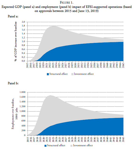
Figure 1.
Expected GDP (panel a) and employment (panel b) impact of EFSI-supported operations (based on approvals between 2015 and June 13, 2019)
Source: RHOMOLO-EIB calculations.
The structural effect impacts the economy according to the profile of the investment. For instance, the effects of transport infrastructure investments for the construction of new transport routes and for the improvement of existing ones are assumed to affect the transport costs in RHOMOLO-EIB. This means that the structural effect of transport infrastructure projects implies a reduction in the bilateral iceberg costs between regions, and the scope of the change can be thought of as a subsidy equivalent. Reduced transport costs change the trade flows and the relative competitiveness of the regional industries, which effects GDP and employment for the regions which experience the reduction in costs. The subsequent changes in imports and exports would also affect welfare and the allocation of the factors of production. Finally, it should be noted that the impact of a better infrastructure would be greater in regions with more potential for trade expansion, such as regions that are already competitive but still lack transport links to reach additional markets. On the other hand, investments in human capital affect the productivity of labour, R&D investments affect total factor productivity, and investments in new capital formation different from transport are assumed to affect capital productivity.
Given the nature of the RHOMOLO-EIB model, results can be analysed under different point of view by exploring both their geographical and their sectorial characteristics. Figure 2 demonstrates that EU regions and countries benefit in terms of jobs and economic growth, on average. When looking at percentage changes, it is clear that the countries that were hit the most by the 2008 economic and financial crisis (the EU periphery), and those lagging behind in terms of income (the cohesion countries), benefited relatively more than the most well-off countries (other countries). This is unsurprising as these countries receive a substantial part of EFSI lending. While the effects cannot be only linked to the level of local investments given the spill overs from one country to the rest, a key explanation lies also in the economic situation of the countries. Many regions in the periphery and cohesion countries experienced relatively high unemployment levels and relative low levels of investments increasing the scope of the investment effects. For the most well-off (other) countries the economic situation after the crisis was different with unemployment levels lower and investments levels typically higher. Hence, the investment effect is more modest and takes longer to pick up.
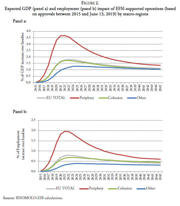
Figure 2.
Expected GDP (panel a) and employment (panel b) impact of EFSI-supported operations (based on approvals between 2015 and June 13, 2019) by macro-regions
Source: RHOMOLO-EIB calculations.
It is equally interesting to look at the sectorial results of the simulations. Figure 3 shows the GDP effects of the EFSI-supported operations on the ten sectors in which the economy is disaggregated in the RHOMOLO-EIB model. In the short term, investments drive up demand which feeds into other sectors of the economy thanks to sectorial spillovers and indirect and induced effects. In the longer term all sectors benefit from the EFSI-supported operations thanks to structural effects. It should be noted that the results should be interpreted as deviations from a reference scenario without EIB interventions, hence, the impact of EFSI on GDP and employment in the manufacturing sector can be positive even if long term structural shift in the economy gradually reduces this sectors share of the economy. Such long-term structural shift in the economy would imply a long-term trend in the sector composition common to both scenarios (with EIB intervention and without EIB intervention). Therefore, the reported impact of EFSI on sectoral GDP and employment does not contain underlying long-term structural shifts in the economy.
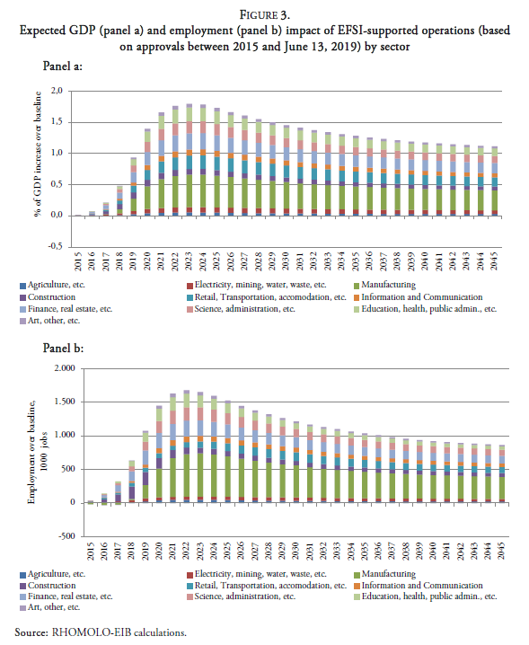
Figure 3.
Expected GDP (panel a) and employment (panel b) impact of EFSI-supported operations (based on approvals between 2015 and June 13, 2019) by sector
Source: RHOMOLO-EIB calculations.
5. Conclusions
This article reports the latest RHOMOLO-EIB results on the macroeconomic impact of EFSI in the EU. After introducing the main features and assumptions of the model, the article focuses on the employment and GDP impact of the EFSI-supported operations approved as of June 13th, 2019 and shows that by 2019 these operations are expected to create more than 1 million jobs over the baseline scenario, which is expected to become 1.7 million by 2022. The estimated contribution to GDP is quantified at 0.9% by 2019, expected to rise to 1.8% by 2022.
The analysis differentiates between investment and structural effects. The former has demand-side macroeconomic effects mainly due to the invested money during the implementation phase of the projects and the financing related to it. The latter affects the economy via the supply-side due to the long-lasting impacts of the EFSI- supported operations on transport costs and productivity.
While the model produces specific results in terms of number of jobs and GDP changes over its baseline, these results provide a sense of scope of the impact of EFSI-supported operations and should not be considered as forecasts. For the avoidance of doubt, while the RHOMOLO-EIB is a version of the well-established RHOMOLO model and therefore its results can be considered robust and credible, other models may deliver different results depending on their baseline calibrations, structure, and main assumptions. The JRC and the EIB Group are committed to continue to analyse the effects of the EFSI-supported operations, to further refine the analysis and conduct thorough sensitivity analysis, and to exploring the impact of additional economic channels (such as cross-regional spillovers).
References
Barro, R.J. (1990). Government spending in a simple model of endogenous growth. Journal of Political Economy 98(5), S103-S125.
Blanchflower, D., & Oswald, A.J. (1994). Estimating a wage curve for Britain 1973-90. The Economic Journal, 0104(426), 1025-1043.
Budzinski, O. (2013). Impact evaluation of merger control decisions. European Competition Journal 9(1): 199-224.
Camisão, I., & Vila Maior, P. (2019). Failure or success: assessing the European Commission’s new strategy to foster EU’s economic recovery. Journal of European Integration.
Christensen, M., Weiers, G., Conte, A., Wolski, M., & Salotti, S. (2019). The European Fund for Strategic Investments: the RHOMOLO-EIB 2019 update. JRC - EIB Territorial Development Insights Series, JRC118260, European Commission.
EIB (2018). Assessing the macroeconomic impact of the EIB Group. Economics - Impact Studies. European Investment Bank, Luxembourg, June.
EU (2015). Regulation (EU) 2015/1017 of the European Parliament and of the Council of 25 June 2015 on the European Fund for Strategic Investments, the European Investment Advisory Hub and the European Investment Project Portal and amending Regulations (EU) No 1291/2013 and (EU) No 1316/2013 - the European Fund for Strategic Investments. Official Journal of the European Union, L, 169: 1-37.
EU (2017). Regulation (EU) 2017/2396 of the European Parliament and of the Council of 13 December 2017 amending Regulations (EU) No 1316/2013 and (EU) 2015/1017 as regards the extension and ruation of the European Fund for Strategic Investments as well as the introduction of technical enhancements for that Fund and the European Investment Advisory Hub. Official Journal of the European Union, L, 345: 34-52.
Fisher, W.H., & Turnovsky, S.J. (1998). Public Investment, Congestion, and Private Capital Accumulation. The Economic Journal , 108(447), 399-413.
Glomm, G., & Ravikumar, B. (1994). Public investment in infrastructure in a simple growth model. Journal of Economic Dynamics and Control , 18(6), 1173-1186.
Glomm, G., & Ravikumar, B. (1997). Productive government expenditures and long-run growth. Journal of Economic Dynamics and Control , 21(1), 183-204.
Lecca, P., Barbero, J., Christensen, M., Conte, A., Di Comite, F., Diaz-Lanchas, J., Diukanova, O., Mandras, G., Persyn, D., & Sakkas, S. (2018). RHOMOLO V3: A spatial modelling framework. JRC Technical Reports JRC111861, EUR 29229 EN. Publications Office of the European Union, Luxembourg.
Lecca, P., Christensen, M., Conte, A., Mandras, G., & Salotti, S. (2019). Upward pressure on wages and the interregional trade spillover effects under demand side shocks. Papers in Regional Science, online https://doi.org/10.1111/pirs.12472.
Nilsson, L. (2018). Reflections on the economic modelling of free trade agreements. Journal of Global Economic Analysis, 3(1), 156-186.
Petersen M.S., Bröcker J., Enei R., Gohkale R., Granberg T., Hansen C.O., Hansen H.K., Jovanovic R., Korchenevych A., Larrea E., Leder P., Merten T., Pearman A., Rich J., Shires J., & Ulied A. (2009). Report on Scenario, Traffic Forecast and Analysis of Traffic on the TEN-T, taking into Consideration the External Dimension of the Union – Final Report, Funded by DG TREN, Copenhagen, Denmark.
Rogelj, J., Den Elzen, M., Höhne, N., Fransen, T., Fekete, H., Winkler, H., Schaeffer, R., Sha, F., Riahi, K., & Meinshausen, M. (2016). Paris Agreement climate proposals need a boost to keep warming well below 2º C. Nature, 534(7609), 631-639.
Sakkas, S. (2018). The macroeconomic implications of the European Social Fund: An impact assessment exercise using the RHOMOLO model. JRC Working Papers on Territorial Modelling and Analysis No. 01/2018, European Commission, Seville, JRC113322.
Thissen M., Ivanova O., Mandras G., & Husby T. (2019). European NUTS 2 regions: construction of interregional trade-linked Supply and Use tables with consistent transport flows. JRC Working Papers on Territorial Modelling and Analysis No. 01/2019, European Commission, Seville, JRC115439.
Turnovsky, S.J., & Fisher, W.H. (1995). The Composition of Government Expenditure and its Consequences for Macroeconomic Performance. Journal of Economic Dynamics and Control , 19(4), 747-786.
Notes
Additional information
JEL classification: C63; C68; E61
Acknowledgment: The authors would like to thank Andrea Conte, Debora Revoltella, Simone Salotti and Jean-Pierre Vidal for helpful inputs.
Corresponding author: Martin.CHRISTENSEN@ec.europa.eu