1. Introduction

Since the seminal papers by North (1990) and Edquist (1997) there is a wide consensus on the idea that institutional quality—or quality of government—matters for economic and social progress. In this vein, the European Union (EU) has engaged quality of institutions as a mean of reduction of regional socio-economic disparities. Following the Copenhagen criteria from 2004,¹ any European state embracing the values of freedom, democracy, equality, rule of law and respect for human rights, as well as a well-functioning market economy, may apply to join the EU. In 2017, the EU Commission recognized tackling widespread corruption and introducing measures aimed at making government decisions more efficient and transparent to be as important as physical investment for regional development (EU Commission, 2017). Accordingly, the implementation of institutional reforms aimed at improving institutional quality can be a valuable tool for regional development strategies.²

Several empirical works have found a positive link between institutional quality and economic performance (e.g. Gwartney et al., 1999; de Haan and Sturm, 2000; Lundstrom, 2005). In particular, the protection of property rights and rule of law are especially relevant in generating sustainable growth (Rodrik et al., 2004; Acemoglu et al., 2005). Nevertheless, despite the abundance of contributions at the country level, or recent studies for particular countries (see Choi, 2018; Quah, 2017), not as many results have been yet delivered addressing regional level analyses on the issue (Rodríguez-Pose, 2013). Some exceptions are found for the European regional context, on which this paper focuses. Crescenzi et al. (2016) found a strong positive relationship between the quality of regional institutions and the returns of infrastructural investments. More similar to the context of our research, Rodríguez-Pose and Garcilazo (2015) disclose local institutional quality to be a vital factor in determining the rate of returns of Cohesion Policy investments. Ketterer and Rodríguez-Pose (2018) found a positive link between institutions and growth for the period 1995-2009 but considered only EU-15 regions. Nonetheless, the topic has become even more important after the latest EU enlargements of 2004, 2007 and 2013, which have remarkably increased development disparities across the Union. Moreover, the new members have institutional quality standards generally below the EU average, as their institutions might be still influenced by the pre-transition institutions, when these countries were ruled by a planned system.

This paper revisits the topic, but differs in several aspects from previous contributions, attempting to provide fresh evidence on this literature. First, it uses a broader and more updated dataset covering the period 2010-2017, including EU-15³ regions and regions from countries that joined the EU after 2004⁴, which might be relevant given the great disparities between these two groups. To date, most of the existent evidence at the regional level corresponds to the pre-crisis years, and it is generally confined to EU-15 regions. Second, we make use of the most recent edition of the European Quality of Government Index (EQI, see Charron et al. 2016; 2019), available for years 2010, 2013 and 2017. In contrast to previous regional analyses mostly relying on a single observation of institutional quality, we are able to analyze its recent evolution by using information from the three years. Charron et al. (2019) introduced the new wave of the EQI index but, to the best of our knowledge, empirical analyses making an effective use of the three waves are still yet to come. Third, we provide a disaggregated analysis for the government quality components, namely quality, impartiality and corruption, which entails the opportunity of delivering more accurate policy implications from the results. Fourth, we address the spatial relationship between government quality and economic growth and quantify the spillover effects.

Based on the previous evidence for Europe and other geographical contexts, we expect a positive relationship between quality of government and economic growth. Also, spatial spillovers are remarkable in European regions (see Ezcurra and Rios, 2019). We therefore expect a notable role of the space in our context. Our results widely support these hypotheses. However, there are some interesting nuances: i) quality of government effects on growth are larger for the EU-15 regions; and ii) generally, clearer effects are found for the components of impartiality and corruption, whereas the effects of the quality component are weaker or non-significant in most models.

The remainder of this paper is structured as follows. In Section 2 we introduce the theoretical foundations and review the relevant literature. The dataset and the descriptive statistics are presented in Section 3. The econometric strategy is described in Section 4. In Section 5 we discuss the main results and, finally, the conclusions and policy implications are summarized in Section 6.

2. Literature review

The influence of institutions on economic development was fundamentally neglected by the mainstream of the economic theory until the nineties. Indeed, the Neoclassical growth models by Solow (1956), as well as the endogenous growth approach developed by Romer (1986) and Lucas (1988), considered economic growth as the result of the mere combination of physical capital, labor, technology and knowledge.

North (1990) suggested that formal institutions matter for economic development, insofar as transactions among individuals in a society are costly. Institutions can be understood as the rules of the game in a society or, more formally, as the humanly devised constraints that shape human interaction. Coherently, the major role of institutions would be that of reducing uncertainty by establishing a stable structure for human cooperation. In this prospective, institutions are bound to influence economic performance as they are capable of reducing transaction costs. Therefore, good institutional settings promote economic development by establishing an environment in which transactions take place under trust and order. Property rights are well-established, and people do not need to devote too many resources to their control and enforcement.

Building on North, numerous studies have highlighted that poor institutional quality makes the economic environment less efficient, entailing lower economic standards. Countries with high corruption, weak rule of law, and low impartiality are associated with, among others, poorer health (Holmberg and Rothstein, 2012), worse environmental outcomes (Welsch, 2004), greater income inequality (Gupta et al. 2002), and even lower levels of happiness (Veenhoven, 2010). Similarly, and more directly addressing our research question, examples of studies reporting a significant relationship between institutional quality and income per capita or income growth include Knack and Keefer (1995), Gwartney et al. (1999), de Haan and Sturm (2000) or Lundstrom (2005). Holmberg et al. (2009) reported positive effects of institutional quality on several welfare dimensions and Mo (2001) found a negative effect of corruption on income growth. There are several mechanisms. First, corruption is associated with less efficiency in the use of the available resources and in the provision of government services because of more inefficient regulations. Moreover, corruption might favor particular elites or social actors, widening economic and social disparities.

Focusing on the European regional context, Crescenzi et al. (2016) study the link between the quality of regional institutions and the rates of returns of infrastructural investments using data for 166 regions between 1995 and 2009. Their research concludes that better institutions lead to higher returns of investment and economic development. Rodríguez-Pose and Di Cataldo (2014) examine the impact of institutional quality on regions’ innovative performance in a sample of 189 EU regions between 1997 and 2009, concluding that there is an institutional quality threshold effect for innovation. Accordingly, policies aimed at improving innovative performance are more likely to be effective in regions where insti­tutional quality is sufficiently high. Nistotskaya et al. (2015) argue that regions where governments are perceived as impartial and free from corruption enjoy a more dynamic economic environment. These effects are found for a sample of 172 regions from 18 EU countries between 1990 and 2007. More recently, Ezcurra and Rios (2019) reported evidence from the last Great Recession, and positively linked quality of government with regional resilience.

More empirical evidence comes from recent studies for the Italian regional context. Lasagni et al. (2015) test the relevance of institutional quality in explaining firm productivity in 107 Italian provinces for the period 1998-2007, finding a key role for the local institutional context. Di Berardino et al. (2019) find that within-country human capital movements are modifying institutional quality, exacerbating the North-South divide in Italy. Coppola et al. (2018) conclude that, whereas quality of government has no implications for EU funds, it increases the impact of subsidies received by firms. Considering a cross-regional European sample, Rodríguez-Pose and Garcilazo (2015) analyze the relationship between insti­tutional quality and the rates of returns of Cohesion Policy investments for a sample of 169 regions for the period 1996-2007, concluding that both EU investments and institutional quality make a difference for regional growth. Additionally, above a certain threshold of expenditure in investments, the quality of institutions becomes the basic factor determining regional growth rates.

From a theoretical point of view, D’agostino and Scarlato (2015) show a positive link between institutional quality and regional economic performance by constructing a three-sector semi-endogenous growth model with negative externalities related to the social and institutional variables affecting the innovative capacity of regional economic systems. Particularly, by applying their model to the Italian regions, they find the enhancement of socio-institutional conditions to be more effective for innovation capacity and economic growth in the lowest-ranked regions in terms of institutional and economic development.

Lastly, as regions are not isolated economic units, spatial spillovers are likely to be important in this context. In this vein, Bologna et al. (2016) show that gains from institutional reforms are not confined to the metropolitan area in which the reforms are enacted, being the effects noticeable in the neighboring regions too.

3. Empirical framework

3.1. The sample

The sample consists of 206 NUTS⁵ 2 European regions from the EU-28. These territorial units are particularly meaningful from a policy perspective as they generally have considerable responsibilities in terms of policy competences, although this varies from one country to another. Throughout the analysis, particular attention will be devoted to the large heterogeneity that characterizes the EU regional economic development and institutional quality standards. To this purpose, two subgroups of regions will be compared: i) regions belonging to countries that were members of the EU prior to the enlargement of 2004 will be referred to as EU-15; ii) regions from countries that joined the EU after that year will be labelled as NMS (New Member States). In the sample, there are 149 EU-15 regions and 57 NMS regions. The dataset covers the period 2010-2017. Such reduced time span was selected due to data constrains in government quality, as the first edition of the EQI index corresponds to 2010.

3.2. Variables, sources and descriptive statistics

As a dependent variable, we use the growth of regional income per inhabitant, expressed in purchas­ing power standards (PPS), taken from Eurostat. This indicator has the advantage of allowing for meaningful comparisons of income by avoiding biases due to discrepancies in purchasing power across European regions. Table 1 summarizes some descriptive statistics for the entire period. The table discloses remarkable differences in both the average GDP per capita and growth rates. As expected, GDP per capita was lower for NMS regions over the studied period; in contrast, they grew faster than the EU-15 group, although disparities between the two groups reduced only slightly.

Government quality is proxied by the European Quality of Government Index (EQI), developed by the Quality of Government Institute - University of Gothenburg (see Charron et al., 2014, 2016, 2019). Data are currently available for years 2010, 2013 and 2017. The EQI index is especially appealing for analyses at the regional level in the European context, as it is based on the same territorial aggregation than most of EU regional statistics, which makes it totally compatible with the information provided by the European Statistical Office (Eurostat) and with the European Regional Policy.⁶

The index defines institutional quality as a multi-dimensional concept consisting of three compo­nents: quality of public services, impartiality and corruption. Specifically, quality and impartiality of regional governments are made out of residents’ ratings of these two characteristics in the areas of public education and health care system, as well as in law enforcement and in the democratic procedures. Analo­gously, residents’ perceptions and experiences with bribery define the indicator for control of corruption. Then, the three components are aggregated to construct a composite index. All the methodological details can be found in the seminal papers by Charron et al. (2014, 2016, 2019), as well as in the Database Codebook, available online.

The original index ranges from -3 to +3, with greater values representing greater government quality. With the aim of simplifying the interpretation of the estimates in the econometric models, we take the min-max normalized values of the variable, which range from 0 to 1,⁷ also provided by the database. Unfortunately, EQI’s observations are not as frequent in time as the rest of the variables in the dataset. Accordingly, the variable is treated as follows. Figures from 2010 are used for observations between 2010 and 2012, those from 2013 are used for observations between 2014 and 2016, and those from 2017 are used for that single year. This approach has an important drawback, as repeated values are assigned to several years. Accordingly, we implement alternative approaches to test for the sensitivity of the results. In particular, we provide results averaging data for the entire period (2010-2017) and for a two-period (2010-2013; 2014-2017) panel structure. Finally, for regions in Belgium, Sweden and Slovenia, government quality is only reported for NUTS 1 units. Then, we assign these scores to the related NUTS 2 units.

Table 1 also shows descriptive statistics for the EQI index. Large disparities are observed between EU-15 and NMS regions, with larger scores for the former group. Similarly, Figure 1 displays the cross-section distribution of the index, both across groups of regions and over time, and shows a decline in government quality, more remarkable between 2010 and 2013. The figure also shows that within-group heterogeneity is high. For example, in the EU-15 group we find regions from Italy, Greece and Spain on the left tail of the distribution, whereas on the right one we find regions from the Nordic countries, Austria and the Netherlands. The densities also suggest that convergence in government quality is not taking place, as their shape is highly persistent.⁸

Table 1.
Descriptive statistics for the main variables

	Average values 2010-2017
	GDP pc(PPS €)		GDP pc growth (%)		EQI index(0-1)
	Mean	S.d.	Mean	S.d.	Mean	S.d.
EU-28	26,134	9,967	0.025	0.014	0.561	0.202
EU-15	29,195	8,861	0.020	0.012	0.638	0.172
NMS	18,132	8,125	0.039	0.011	0.360	0.123

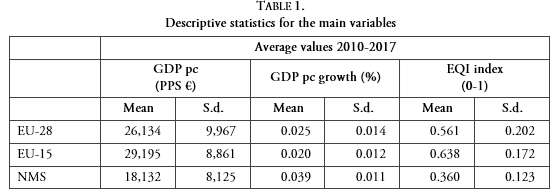
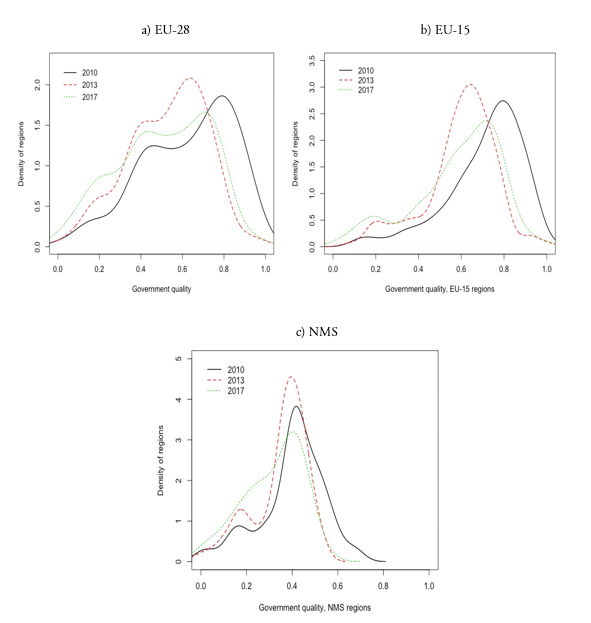
Figure 1.
Kernel densities for government quality (EQI index)

The dataset provides disaggregated information for the three components of the EQI index: quality, impartiality and corruption. Table 2 reports information for these indicators for years 2010, 2013 and 2017. Similarly to what is found for the aggregated index, a decline is observable between 2010 and 2013. In contrast, in 2017 impartiality and quality improved, while corruption levels worsened even more for the EU-15 group. In the NMS group corruption remained relatively stable. Considering the entire sample (EU-28), the components of quality, impartiality and corruption declined by 10.6%, 10.2% and 14%, respectively, between 2010 and 2017.⁹

Table 2.
Evolution of the government quality components

	Quality			Impartiality			Corruption
	2010	2013	2017	2010	2013	2017	2010	2013	2017
EU-28	0.655	0.529	0.585	0.637	0.556	0.572	0.605	0.555	0.520
EU-15	0.713	0.579	0.639	0.704	0.602	0.624	0.673	0.616	0.568
NMS	0.472	0.375	0.413	0.439	0.406	0.408	0.402	0.364	0.367

As control variables we include the classical Solow variables, extensively used in the growth literature. We followed the seminal contributions by Barro (1991), Mankiw et al. (1992) and also more recent studies such as Crespo-Cuaresma et al. (2014), focused on the European context. The use of the Solow framework and Barro-type growth equations as a starting point when evaluating other theories in growth empirics is today widely supported (e.g. Durlauf et al. 2008; Henderson et al. 2012).¹⁰

Our first control is the initial level of GDP per capita, in our case year 2010. A negative coefficient would imply that conditional convergence is taking place, i.e. subject to other regional fundamentals, poorer regions grow faster than the richer ones. The rest of controls include the annual R&D investments as share of GDP, treated as a proxy of technological progress. Labor and physical capital are included into the model through the regional population growth rate and the gross fixed capital formation (share of GDP), respectively. Moreover, as a proxy of human capital, the percentage of highly educated workers (tertiary education) is also considered (see Dettori et al. 2012). Data for all these controls are provided by Eurostat. Finally, following Crespo-Cuaresma et al. (2014), qualitative features are also controlled for by means of two dummy variables. The variable “NMS” takes the value of 1 if the region belongs to the NMS group and 0 otherwise, while the variable “capital city” takes the value of 1 when a region hosts the country’s capital city within its borders and 0 otherwise. Capital cities are generally a suitable environment for companies’ economic activities because of urban agglomeration and economic dynamism. Therefore, this qualitative characteristic is expected to have a positive role in explaining regional growth.

4. Econometric strategy

We estimate several model specifications, differing in the controls included. In some models, we also include interactions between government quality and the dummy variable NMS in order to study whether different impacts are found between groups. The most general model takes the form:

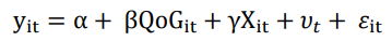(1)

where the subscripts and represent a given region and year, respectively, is regional output per capita growth, represents either government quality or each of its three components, is a vector of control variables and stands for time effects. Finally, and are the model parameters and is the error term. The models are first estimated via Ordinary Least Squares (OLS).

Additionally, we consider several strategies to control for spatial spillovers. Given that the presence of unattended spatial spillovers in the data might produce non-robust estimates, testing for the existence of spatial dependence in our models is highly advisable. First, we run the Pesaran’s (2004) test, which assesses in a panel data context the cross-sectional dependence of the residuals in the OLS models. After verifying this is actually the case (the null hypothesis of no cross-sectional dependence is rejected in all cases), we model the spatial effects by means of specific spatial models. Following Elhorst (2010) and LeSage and Pace (2009) we first run a Spatial Durbin Model (SDM), able to control for spatial spillovers in both the dependent and the independent variables. Formally:

(2)

where 𝑖 and 𝑗 are two given regions, 𝜌, η and 𝛿𝛿 are the spatial parameters and 𝑊 is a matrix of spatial weights describing the neighboring relationship between regions. The rest of elements are common to Equation (1). To construct the 𝑊 matrix, the inverse distance is first computed between all 𝑖𝑖 pairs. Then, the 𝑘-nearest neighbor criterion is followed, which considers the 𝑘 closest regions to the geographical unit of interest as its neighbors. Although all the criteria to define the 𝑊 matrix are debatable, growth determinants in the European regional context are not particularly affected by different specifications of the neighbor matrix. Crespo-Cuaresma et al. (2014) found analogous results using both distance-based and contiguity matrices, highlighting that the latter might capture regional spillovers appropriately. Also, LeSage (2014) postulated in favor of contiguity matrices, claiming the importance of setting a cut-off distance beyond which weights are zero and arguing that results from spatial models are relatively robust to changes in 𝑊. Following these arguments, pairs of neighbors in 𝑊 are represented by ones, while the rest of pairs take the value of zero. Moreover, following the standard convention, we row-normalize 𝑊 such that its rows sum one. Accordingly, elements in 𝑊 are defined as follows:

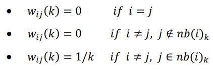
where stands for the specific spatial link between regions and and refers to the neighborhood of region for a given . Given that EU NUTS 2 regions have generally from three to seven contiguous regions, we set as a rule of neighboring.

Following the general-to-specific strategy proposed by Elhorst (2010), it is advisable to test whether the more comprehensive SDM can be simplified into a Spatial Lag Model—also known as Spatial Autoregressive Model (SAR), with spatial spillovers only in the dependent variable, or into a Spatial Error Model (SEM), with the spatial autocorrelation embedded in the error term. Formally, the SAR and SEM models are represented by Equations 3 and 4, respectively:

(3)

(4)

where , and are disturbances and the parameters and summarize the strength of the spatial dependence. Despite models involving global spillover processes such as the SDM and the SAR have been criticized in growth contexts (see Corrado and Fingleton, 2012; Halleck-Vega and Elhorst, 2015), the literature is still inconclusive on this point.^[11] In fact, other authors including Ertur and Koch (2007), Fischer (2011), D’agostino and Scarlato (2015) or Fiaschi et al. (2018) argue that these models can correctly capture technological and learning externalities, which are well-known growth drivers. Another example is Crespo-Cuaresma et al. (2014), who based their analysis of growth determinants for the European regions on SAR estimations. All the spatial models are estimated via Maximum Likelihood (MLE).

5. Results

5.1. Baseline estimations

According to the theoretical arguments, we expect positive coefficients for government quality (North,1990), education and R&D investment (Dettori et al. 2012) and the dummies for capital city and NMS group (Crespo-Cuaresma et al. 2014). It is more difficult to forecast the sign for physical capital investment, as it can be generally more effective in developing economies. In our sample, despite the income heterogeneity, all regions are relatively developed (see Crespo-Cuaresma et al. 2014). Finally, in accordance with the theory of beta convergence, the initial level of regional income per capita is expected to exert a negative impact on the dependent variable. The same sign is expected for population growth.

Models 1 to 7 in Table 3 combine fixed and random effects estimations with different control variables. Although quality of government is not significantly associated to growth in Models 1 to 3, once important control variables such as R&D investment, capital city and especially the dummy variable NMS are included, its coefficient adopts the expected positive and significant effect. One potential explanation is that the different levels of quality of government and growth rates between former and new EU members may mask the effect of quality of government when the dummy variable is omitted.

Model 6 incorporates the interaction between government quality and the NMS dummy. A negative sign is obtained and, accordingly, government quality has a larger effect on growth in EU-15 regions. As NMS regions grew faster despite their comparatively lower government quality and the main effect for government quality remains positive—in fact this is the model yielding the largest coefficient—NMS regions are losing an important growth potential.¹² In other words, both their comparatively lower government quality and the lower capacity of their institutions to generate growth are slowing down their catching-up process with the EU-15. Given the interest of the European policymakers in reaching conver­gence, this has implications for the design of future policies. Despite the new members are slowly catching-up, there is a long way until they could reach the GDP per capita levels of the former EU-15 group. Strengthen the quality of their institutions could be an appropriate strategy to reduce the gap but, unfor­tunately, what we are actually witnessing is a general decline of government quality across the entire EU-28 in recent years.

Regarding the control variables, the initial level of income per capita is negative only when the NMS dummy is not included. Logically, when this variable is added, it captures the effect of the initial GDP, as the NMS coefficient is clearly positive (note that NMS regions have lower initial income levels). Population growth is negative in all cases, in line with the previous literature. More controversial are the results found for education, generally non-significant across models. In contrast, R&D investment exhibits a positive sign in all of them. We argue that this latter variable can be partially absorbing the effect of education, as they are positively correlated—higher R&D efforts take place in regions with more qualified labor force. The effect of physical capital investment is non-significant, indicating that growth in the analyzed period is more driven by knowledge and institutional factors than by physical investment.

Finally, in Model 7 we run a fixed effects estimation with all the controls. Unfortunately, this procedure removes all the time invariant variables, including the dummy variable for NMS regions, in which we are interested. When comparing fixed and random models with the Hausman test, we are unable to compare the models including the time invariant controls. The test was performed for Model 4 and for that specification the fixed effects alternative was preferable. However, few clear insights can be obtained from the fixed effects estimation in Model 7, as only population growth remains significant, which are results difficult to reconcile with the well-stablished growth theory. In addition, as the NMS dummy becomes part of the fixed effects, we cannot test whether different impacts are found for these regions, as we do in Model 6. If the predominant source of variation is cross-regional instead of within-regional, which is our case, fixed effects estimations can be troublesome and produce inaccurate results (Barro, 2000; Partridge, 2005). The cross-regional variation of the EQI index is notably larger than that within-regional,¹³ thus explaining in a large extent the puzzling results from the fixed effects models. In contrast, random effects models perform similarly to OLS cross-sectional models.

Given the particularities of our data, we prefer the random effects alternative for the subsequent analyses, even at the cost of assuming that, once initial GDP per capita and NMS are included in the model, the explanatory variables are not systematically correlated with the error term. Of course, this is debatable, but we consider ours as a balanced strategy given the counterintuitive results from the fixed effect models. Finally, Table 4 contains separate results for the three components of government quality using the most comprehensive specification and random effects estimations. The results suggest that all three components are positive and significant. In addition, their interaction with the dummy NMS is negative, in line with the results found for the aggregated indicator in Table 3. This corroborates the comparatively lower impact of government quality on growth in NMS regions.

Table 3.
Government quality and GDP per capita growth

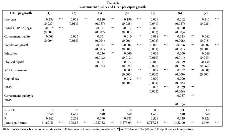
All the models include but do not report time effects. Robust standard errors are in parentheses. *, ** and *** denote 10%, 5% and 1% significant levels, respectively.

GDP pc growth	(1)		(2)		(3)		(4)		(5)		(6)		(7)
Intercept	0.186	***	0.054	**	0.140	***	0.199	***	0.024		0.012		0.115	***
	(0.027)		(0.011)		(0.027)		(0.028)		(0.036)		(0.037)		(0.021)
Initial GDP pc (logs)	-0.015	***			-0.011	***	-0.017	***	-0.000		0.000
	(0.002)				(0.002)		(0.002)		(0.003)		(0.003)
Government quality	0.003		-0.029		0.001		0.010	*	0.018	***	0.025	***	-0.042
	(0.005)		(0.019)		(0.005)		(0.006)		(0.005)		(0.006)		(0.018)
Population growth					-0.007	***	-0.007	***	-0.006	***	-0.006	***	-0.007	***
					(0.001)		(0.001)		(0.001)		(0.001)		(0.001)
Education					0.026	**	-0.000		0.005		0.000		-0.049
					(0.012)		(0.012)		(0.010)		(0.011)		(0.049)
Physical capital					0.011		0.017		-0.016		-0.019		-0.144
					(0.024)		(0.024)		(0.022)		(0.019)		(0.060)
R&D investment							0.002	**	0.002	***	0.002	***	-0.005
							(0.000)		(0.000)		(0.000)		(0.005)
Capital city							0.012	***	0.000		0.000
							(0.004)		(0.004)		(0.005)
NMS									0.023	***	0.039	***
									(0.003)		(0.006)
Government quality x NMS											-0.037	***
											(0.013)
RE / FE	RE		FE		RE		RE		RE		RE		FE
N	1,648		1,648		1,648		1,648		1,648		1,648		1,648
R2	0.242		0.204		0.270		0.285		0.324		0.329		0.126
Joint significance	1,162.41	***	106.12	***	1,287.32	***	1,273.03	***	1,717.28	***	1,622.10	***	89.94	***

Table 4.
Government quality components and GDP per capita growth

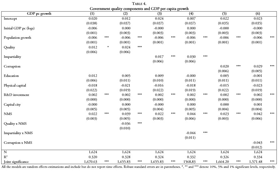
All the models are random effects estimations and include but do not report time effects. Robust standard errors are in parentheses. *, ** and *** denote 10%, 5% and 1% significant levels, respectively.

GDP pc growth	(1)		(2)		(3)		(4)		(5)		(6)
Intercept	0.020		0.012		0.024		0.007		0.022		0.023
	(0.038)		(0.037)		(0.037)		(0.037)		(0.035)		(0.035)
Initial GDP pc (logs)	-0.006		0.000		-0.000		0.000		-0.000		-0.000
	(0.001)		(0.003)		(0.003)		(0.003)		(0.003)		(0.003)
Population growth	-0.006	***	-0.006	***	-0.006	***	-0.006	***	-0.006	***	-0.006	***
	(0.001)		(0.001)		(0.001)		(0.001)		(0.001)		(0.001)
Quality	0.012	*	0.024	***
	(0.006)		(0.006)
Impartiality					0.017	***	0.030	***
					(0.006)		(0.006)
Corruption									0.020	***	0.029	***
									(0.006)		(0.005)
Education	0.012		0.005		0.009		-0.000		0.005		-0.001
	(0.006)		(0.011)		(0.010)		(0.011)		(0.011)		(0.011)
Physical capital	-0.018		-0.021		-0.016		-0.018		-0.015		-0.023
	(0.022)		(0.019)		(0.022)		(0.019)		(0.022)		(0.019)
R&D investment	0.002	***	0.002	***	0.002	***	0.002	***	0.002	***	0.002	***
	(0.000)		(0.000)		(0.000)		(0.000)		(0.000)		(0.000)
Capital city	-0.000		0.000		-0.000		0.000		0.000		0.001
	(0.005)		(0.005)		(0.004)		(0.005)		(0.004)		(0.004)
NMS	0.022	***	0.039	***	0.022	***	0.044	***	0.023	***	0.042	***
	(0.003)		(0.005)		(0.003)		(0.006)		(0.003)		(0.006)
Quality x NMS			-0.036	***
			(0.010)
Impartiality x NMS							-0.044	***
							(0.011)
Corruption x NMS											-0.043	***
											(0.012)
N	1,624		1,624		1,624		1,624		1,624		1,624
R2	0.320		0.328		0.324		0.332		0.326		0.334
Joint significance	1,670.63	***	1,655.83	***	1,655.83	***	1568,83	***	1,664.20	***	1,571.48	***

5.2. Spatial spillovers

This section details the results from the spatial models, reported in Table 5. As explained in Section 4, the neighboring W matrix was specified using the k-nearest neighbor criterion, setting k=5. The Pesaran’s (2004) tests (available at the bottom of the table) point to the existence of spatial dependence in the residuals of the non-spatial (OLS) estimations. After detecting the spatial autocorrelation, we estimate SDM models. As argued by LeSage and Pace (2009), SDM can provide unbiased estimates even if the true model is a SEM or a SAR.¹⁴ Therefore, it is a wise starting point.

Table 5.
SAR estimations for government quality and GDP per capita growth

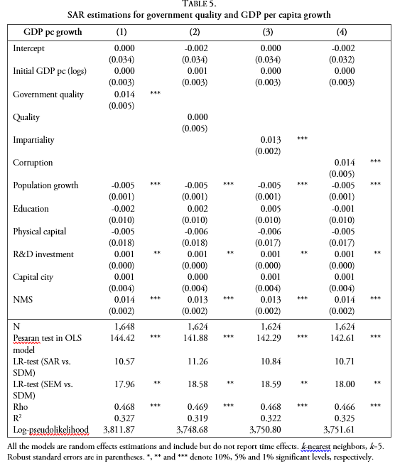
All the models are random effects estimations and include but do not report time effects. k-nearest neighbors, k=5. Robust standard errors are in parentheses. *, ** and *** denote 10%, 5% and 1% significant levels, respectively.

GDP pc growth	(1)		(2)		(3)		(4)
Intercept	0.000		-0.002		0.000		-0.002
	(0.034)		(0.034)		(0.034)		(0.032)
Initial GDP pc (logs)	0.000		0.001		0.000		0.000
	(0.003)		(0.003)		(0.003)		(0.003)
Government quality	0.014	***
	(0.005)
Quality			0.000
			(0.005)
Impartiality					0.013	***
					(0.002)
Corruption							0.014	***
							(0.005)
Population growth	-0.005	***	-0.005	***	-0.005	***	-0.005	***
	(0.001)		(0.001)		(0.001)		(0.001)
Education	-0.002		0.002		0.005		-0.001
	(0.010)		(0.010)		(0.010)		(0.010)
Physical capital	-0.005		-0.006		-0.006		-0.005
	(0.018)		(0.018)		(0.017)		(0.017)
R&D investment	0.001	**	0.001	**	0.001	**	0.001	**
	(0.000)		(0.000)		(0.000)		(0.000)
Capital city	0.001		0.000		0.001		0.001
	(0.004)		(0.004)		(0.004)		(0.004)
NMS	0.014	***	0.013	***	0.013	***	0.014	***
	(0.002)		(0.002)		(0.002)		(0.002)
N	1,648		1,624		1,624		1,624
Pesaran test in OLS model	144.42	***	141.88	***	142.29	***	142.61	***
LR-test (SAR vs. SDM)	10.57		11.26		10.84		10.71
LR-test (SEM vs. SDM)	17.96	**	18.58	**	18.59	**	18.00	**
Rho	0.468	***	0.469	***	0.468	***	0.466	***
R2	0.327		0.319		0.322		0.325
Log-pseudolikelihood	3,811.87		3,748.68		3,750.80		3,751.61

However, it is also advisable to test whether the SDM can be simplified into a SEM or a SAR (Elhorst, 2010). Then, we perform likelihood ratio tests (LR-tests, also available at the bottom of Table 5). The results indicate that the SAR model cannot be rejected in front of the SDM, while the SEM is rejected in all cases. We therefore report the SAR models in Table 5, as this is the preferred specification.

We find positive estimated coefficients for government quality. When focusing on the individual components, positive effects are found for impartiality and corruption, whereas a non-significant coeffi­cient is obtained for the quality component. Analogously, the rest of the explanatory variables also disclose consistent coefficients with the results previously discussed. The average spatial autocorrelation is summarized by the Rho coefficient, around 0.46 in all the models and indicating a highly positive spatial autocorrelation.

In order to interpret the coefficients from the SAR model, direct and indirect impacts need to be computed, as these models generate spatial spillovers (see, for technical details LeSage and Pace, 2009). Then, changes in government quality in one region not only affect growth in that region, but also growth in its neighbors. Finally, the growth of the neighbors will have a positive feedback effect on the region where initially the variation in government quality took place, giving rise to the direct effect. In contrast, the indirect effect is the average impact of changes in government quality in one region on its neighbors’ growth. The results are reported in Table 6. Interestingly, whereas the components of impartiality and corruption exhibit very similar impacts to those for the aggregated index, the effects for the quality component are non-significant. In terms of size, we find that the indirect effects are almost as large as the direct ones, indicating that the spatial spillovers play a remarkable role and should be taken into account. The total effects are the sum of both direct and indirect impacts.

Table 6.
Direct, indirect and total effects of government quality on GDP per capita growth

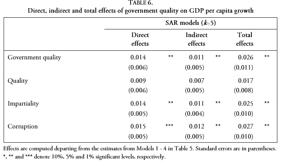
Effects are computed departing from the estimates from Models 1 - 4 in Table 5. Standard errors are in parentheses. *, ** and *** denote 10%, 5% and 1% significant levels, respectively.

	SAR models (k=5)
		Directeffects		Indirect effects		Total effects
Government quality		0.014	**	0.011	**	0.026	**
		(0.006)		(0.005)		(0.011)
Quality		0.009		0.007		0.017
		(0.006)		(0.005)		(0.008)
Impartiality		0.014	**	0.011	**	0.025	**
		(0.005)		(0.004)		(0.010)
Corruption		0.015	***	0.012	**	0.027	**
		(0.005)		(0.005)		(0.010)

5.3. Robustness tests

Different techniques are employed to check for the robustness of the results. First, given that we used repeated figures of quality of government for the intermediate years, we replicate the main models for different time periods. Table A1 in the Appendix A provides the results. In the table, columns (1) to (5) correspond to a cross-sectional framework, in which we average all the available information for the period 2010-2017. Columns (6) to (10) contain the results of a two-period panel data estimation. The first period averages all the time-varying information of years 2010-2013 and uses government quality data from 2010. The second period averages the time-varying data of years 2014-2017, while government quality is the average of the two available figures for that period, namely 2013 and 2017. The results are in all cases in line with the baseline estimations of Tables 3 and 4, both in terms of size of the coefficients and significance levels.

Second, with respect to the spatial analysis, the regressions are performed using different neighboring criteria, namely k=3 and k=7, that is, considering as neighbors the three and seven nearest regions, respec­tively. The results are reported in Table A2 of the Appendix A and are qualitatively analogous to those obtained with k=5. The quality component is non-significant or only weakly significant, whereas positive and significant coefficients, almost identical in size regardless of the matrix used, are found for impartiality and corruption.

6. Concluding remarks and policy prescriptions

This paper has assessed the role of government quality on European regional growth for the period 2010-2017. The findings largely support North’s (1990) proposition according to which institutions drive economic performance, hence resulting as a valuable tool for achieving regional progress. In the framework of the European Regional Policy, this means that government quality should become an important tool to achieve regional convergence. Our analysis has shown that regions from the new EU members (NMS) have remarkably lower levels of government quality than the former EU-15 economies. Consequently, although the new members are growing comparatively faster, their low-quality institutions are decelerating the catching-up process. We argue that institutions need some time to improve. The NMS economies have completed the transition from a planned to a free market economy but, it is possible that their insti­tutional frameworks have still reminiscences from the burdensome and inefficient institutional apparatus of the communist system.

Our results point to a positive role of government quality on economic growth, which is coherent with the previous findings by Rodríguez-Pose and Garcilazo (2015), Crescenzi et al. (2016) and Ketterer and Rodríguez-Pose (2018). With respect to the previous literature, we provide results for a more recent period of time. Also, we used richer information, as we considered the three available editions of the EQI index (2010, 2013 and 2017), analyzed individual components, and quantified spatial spillovers.

The data show a decline in government quality across all the EU-28, similar in size in both the EU-15 and the NMS groups. Then, the institutional distance between the two groups remained relatively stable over the studied period. Accordingly, policy efforts should be addressed to improve government quality all across the Union, with special emphasis in narrowing the gap between former and new members. In addition, the results from the spatial panel approach reveal the existence of positive feedback effects, implying the presence of virtuous reciprocal influences between neighbor regions. The results for govern­ment components provide additional clues on where policies should put the effort. In particular, once spatial spillovers are considered, having highly impartial and corruption-free institutions are those elements more directly related to growth. In contrast, a weaker or even a non-significant effect is found for the quality of government services.

In the light of our findings, some policy advices aimed at improving regional economic performance through government quality are presented. For instance, Alesina (2003) suggested that subnational administrations exerting their powers in smaller territories generally have to deal with less heterogeneous individual preferences. This feature would allow local governments to supply public policies that are closer to residents’ preferences and increase their efficiency. Then, government reforms aimed at decentralizing the executive power and at establishing a clearer separation of the duties between central and subnational governments should be encouraged.

Other authors such as Padovano and Ricciuti (2009) found that higher competitiveness in the political arena improves the quality of local institutions. Thus, measures aimed at increasing democratic competitiveness and alternation between political forces, such as setting limits to the mandates of regional governors might be considered as well. This could help in improving the impartiality and the corruption components. All in all, institutions should be considered not always as a provider, but also as the object of public policies.

Finally, it must be acknowledged that the paper has also some limitations. One derives from the nature of the data on government quality, for which yearly information is not available. We attempted to address this issue by artificially assigning repeated values to intermediate years or averaging the data for different periods. Despite we obtain very similar results when using different temporal aggregations, results should be taken cautiously. Another important limitation is the potential existence of endogeneity, which is not treated in the paper and might be a promising avenue for future research.

Acknowledgments

Acknowledgements I am grateful to the Spanish Ministry of Economy and Competitiveness (project ECO2017-85746-P) and the University Jaume I (project UJI-B2017-33) for financial support.

References

Acemoglu, D., Johnson, S., & Robinson, J. (2005). Institutions as a fundamental cause of long–run growth. In P. Aghion, & S. Durlauf, Handbook of Economic Growth. North Holland, Amsterdam.

Alesina, A. (2003). The size of countries: does it matter? Journal of the European Economic Association, 1(2), 301-316.

Barro, R. (1991). Economic growth in a cross section of countries. The Quarterly Journal of Economics, 106(2), 407-443.

Barro, R. (2000). Inequality and growth in a panel of countries, Journal Economic Growth5, 5–32.

Basyal, D.K., Poudyal, N., & Seo, J.W. (2018). Does E‐government reduce corruption? Evidence from a heterogeneous panel data model, Transforming Government: People, Process and Policy, 12 (2),134‐154.

Bologna, J., Young, A.T., & Lacombe, D.J. (2016). A spatial analysis of incomes and institutional quality: evidence from US metropolitan areas. Journal of Institutional Economics, 12 (1), 191-216.

Charron, N., Dijkstra, L., & Lapuente, V. (2014). Regional governance matters: Quality of government within European Union Member States. Regional Studies, 48(1), 68-90.

Charron, N., Dahlberg, S., Holmberg, S., Rothstein, B., Khomenko, A., & Svensson, R. (2016). The Quality of Government EU Regional Dataset, version Sep16. University of Gothenburg: The Quality of Government Institute, http://www.qog.pol.gu.se

Charron, N., Lapuente, V., & Annoni, P. (2019). Measuring quality of government in EU regions across space and time. Papers in Regional Science, forthcoming.

Choi, J.W. (2018). Corruption control and prevention in the Korean government: Achievements and challenges from an institutional perspective, Asian Education and Development Studies, 7 (3), 303‐314.

Coppola, G., Destefanis, S., Marinuzzi, G., & Tortorella, W. (2018). European Union and nationally based cohesion policies in the Italian regions. Regional Studies, forthcoming.

Corrado, L., & Flingleton, B. (2012). Where is the Economics in Spatial Econometrics?. Journal of Regional Science, 52, 210-239.

Crescenzi, R., Di Cataldo, M., & Rodríguez-Pose, A. (2016). Government quality and the economic returns of transport infrastructure investment in European regions. Journal of Regional Science, 56(4), 555-582.

Crespo-Cuaresma, J., Doppelhofer, G., & Feldkircher, M. (2014). The determinants of economic growth in European regions. Regional Studies, 48(1), 44-67.

D'agostino, G., & Scarlato, M. (2015). Innovation, socio-institutional conditions and economic growth in the Italian regions. Regional Studies, 49(5), 555-582.

de Haan, J., & Sturm, J.E. (2000). On the relationship between economic freedom and economic growth. European Journal of Political Economy, 16(2), 215-241.

Dettori B., Marrocu, E., & Paci, R.R. (2012). Total factor productivity, intangible assets and spatial dependence in the European regions. Regional Studies, 46(10), 1401-1416.

Di Berardino, C., D'Ingiullo, D., Quaglione, D., & Sarra, A. (2019). Migration and institutional quality across Italian provinces: The role of human capital. Papers in Regional Science, 98, 843–860.

Durlauf, S.N., & Quah, D.T. (1999). The new empirics of economic growth. In U. Taylor, Handbook of Macroeconomics. North Holland.

Durlauf, S.N., Kourtellos, A., & Ming Tan, C. (2008). Are any growth theories robust? The Economic Journal, 118(527), 329-346.

Edquist, C. (1997). Systems of Innovation: Technologies, Institutions, and Organizations. London: Cassell Academic.

Elhorst, J.P. (2010), Applied Spatial Econometrics: Raising the Bar, Spatial Economic Analysis, 5(1), 9-28.

European Commission. (2017). Seventh Report on Economic, Social and Territorial Cohesion. Luxembourg: Publications Office of the European Union.

Ertur, C., & Koch, W. (2007). Growth, technological interdependence and spatial externalities: Theory and evidence. Journal of Applied Econometrics, 22(6), 1033-1062.

Ezcurra, R., & Rios, V. (2019). Quality of government and regional resilience in the European Union. Evidence from the Great Recession. Papers in Regional Science, forthcoming.

Fiaschi, D., Lavezzi, A. M., & Parenti, A. (2018). Does EU cohesion policy work? Theory and evidence. Journal of Regional Science , 58(2), 386-423.

Fischer, M. M. (2011). A spatial Mankiw-Romer-Weil model: theory and evidence. The Annals of Regional Science, 47(2), 419-436.

Gupta, S., Davoodi, H., & Alonso-Terme, R. (2002). Does corruption affect income inequality and poverty? Economics of Governance, 3(1), 23-45.

Gwartney, J. D., Lawson, R., & Holcombe, R. G. (1999). Economic freedom and the environment for economic growth. Journal of Institutional and Theoretical Economics, 155(4), 643-663.

Halleck-Vega, S., & Elhorst, J.P. (2015). The SLX Model. Journal of Regional Science, 55(3), 339-363.

Henderson, D. J., Papageorgiou, C., & Parmeter, C. F. (2012). Growth empirics without parameters. Economic Journal 122(559):125–154.

Holmberg, S., Rothstein, B., & Nasiritousi, N., (2009). Quality of government: What you get. Annual Review of Political Science12, 135-161.

Holmberg, S., & Rothstein, B. (2012). Good Government: the Relevance of Political Sciences. Cheltenham: Edward Elgar Publishing Limited.

Ketterer, T.D., & Rodríguez-Pose, A. (2018). Institutions vs. ‘first-nature’ geography: What drives economic growth in Europe’s regions? Papers in Regional Science, 97 (S1), 25-62.

Knack, S., & Keefer, P., (1995). Institutions and economic performance: Cross-country tests using alternative institutional measures. Economics & Politics7(3), 207-227.

LeSage, J.P. (2014). What regional scientists need to know about spatial econometrics, The Review of Regional Studies, 44, 13-32.

LeSage, J.P., & Pace, R.K. (2009). An introduction to Spatial Econometrics. Chapman and Hall/CRC. New York.

Lasagni, A., Nifo, A., & Vecchione, G. (2015). Firm productivity and institutional quality: evidence from Italian industry. Journal of Regional Science, 55(5), 774-800.

Lucas, R. (1988). On the mechanics of economic development. Journal of Monetary Economics, 22(1), 3-42.

Lundstrom, S. (2005). The effect of democracy on differente categories of economic freedom. European Journal of Political Economy, 21(4), 967-980.

Mankiw, G., Romer, D., & David, N. (1992). A contribution to the empirics of economic growth. The Quarterly Journal of Economics, 107(2), 407-437.

Mo, P.H. (2001). Corruption and economic growth. Journal of Public Economics29, 66–79.

Nistotskaya, M., Charron, N., & Lapuente, V. (2015). The wealth of regions: quality of government and SMEs in European regions. Evironment and Planning C: Government and Policy, 33(5), 1125-1155.

North, D. (1990). Institutions, Institutional Change, and Economic Performance. Cambridge: Cambridge University Press.

Partridge, M. D. (2005). Does income distribution affect U.S. state economic growth?, Journal of Regional Science, 45(2), 363–394.

Padovano, F., & Ricciuti, R. (2009). Political competition and economic performance: evidences from Italian provinces. Public Choice, 138(3), pp. 263-277.

Peiró-Palomino, J. (2016). Social capital and economic growth in Europe: nonlinear trends and heterogeneous regional effects, Oxford Bulletin of Economics and Statistics, 78 (5), 717-751

Pesaran, M.H. (2004). General Diagnostic Tests for Cross Section Dependence in Panels. IZA Discussion Paper No. 1240

Quah, J.S.T. (2017). Learning from Singapore’s effective anti‐corruption strategy: Policy recommendations for South Korea, Asian Education and Development Studies, 6(1), 17‐29.

Rodrick, D., Subramanian, A., & Trebbi, F. (2004). Institutions rule: the primacy of institutions over geography and integration in economic development. Journal of Economic Growth, 9(2),131-165.

Rodríguez-Pose, A. (2013). Do institutions matter for regional economic development? Regional Studies, 47(7), 1034-1047.

Rodríguez-Pose, A., & Di Cataldo, M. (2014). Quality of government and innovative performance in the regions of Europe. Journal of Economic Geography, 15(4), 673-706.

Rodríguez-Pose, A., & Garcilazo, E. (2015). Quality of government and returns of investments: Examining the impact of cohesion expenditure in European regions. Regional Studies, 49(8), 1274-1290.

Romer, P. (1986). Increasing returns and long-run growth. Journal of Political Economy, 94(5), 1002-1037.

Solow, R. (1956). A contribution to the theory of economic growth. Quarterly Journal of Economics, 70(1), 65-94.

Veenhoven, R. (2010). How universal is happiness? In E. Diener, J. Helliwell, & D. Kahneman, International Differences in Well-being. Oxford University Press.

Welsch, H. (2004). Corruption, growth and environment: A cross-country analysis. Environment and Development Economics, 9(5), 663-693.

Appendix A. Robustness tests

Table A1
Results for different periods

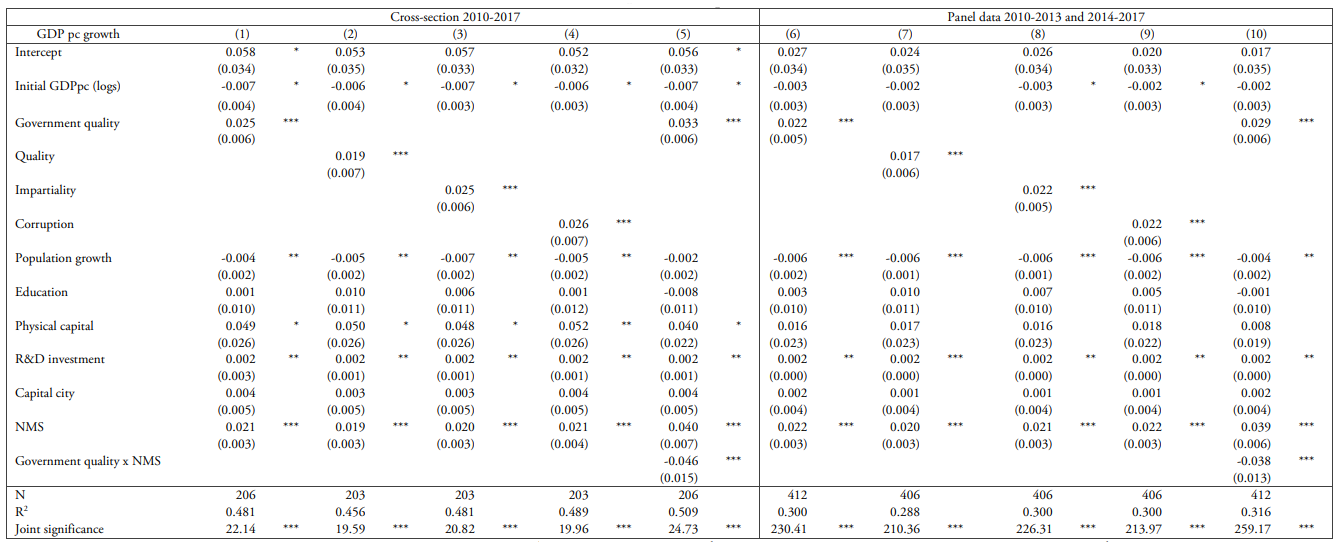
Columns (1) to (5) correspond to a cross-section analysis averaging all the available data in the period 2010-2017. Columns (6) to (10) correspond to a two-period panel analysis, averaging the available data for periods (2010-2013) and (2014-2017). Panel data models are random effects estimations and include but do not report time effects. Robust standard errors are in parentheses. *, ** and *** denote 10%, 5% and 1% significant levels, respectively.

Table A2
SAR estimations with alternative specifications of the spatial matrix (k=3 and k=7)

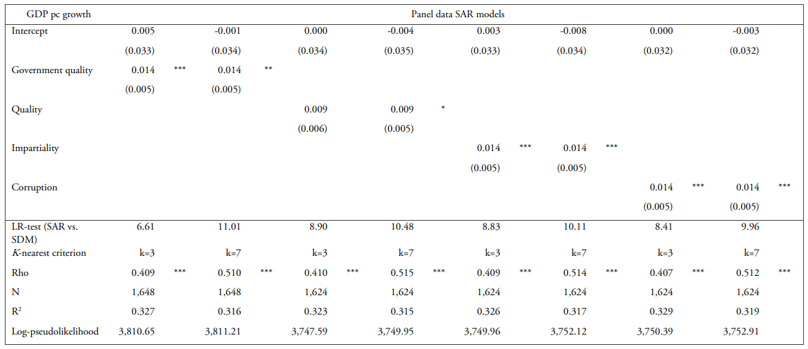
All the models are random effects estimations and include but do not report time effects and control variables. Robust standard errors are in parentheses. *, ** and *** denote 10%, 5% and 1% significant levels, respectively.

Notes

Información adicional

JEL classification: O43; R11; R50.

Corresponding author: jesus.peiro@uv.es

Acknowledgements: I am grateful to the Spanish Ministry of Economy and Competitiveness (project ECO2017-85746-P) and the University Jaume I (project UJI-B2017-33) for financial support.