Articles
The changing geographies of fertility in Spain (1981-2018)
The changing geographies of fertility in Spain (1981-2018)
Investigaciones Regionales - Journal of Regional Research, vol. 2021/2, núm. 50, pp. 147-167, 2021
Asociación Española de Ciencia Regional

Esta obra está bajo una Licencia Creative Commons Atribución-NoComercial 4.0 Internacional.
Recepción: 24 Abril 2020
Aprobación: 03 Mayo 2021
Abstract:
The objective of this article is to investigate the variation of fertility across Spain’s geographic areas between 1981 and 2018, to highlight spatial change over three decades of major fertility transformations. During the last decades, Spanish fertility decreased considerably to below replacement levels. Although total fertility remains below replacement level in Spain, there are important differences in subnational trends that seem to concentrate around certain areas. Starting from the assumption that there is fertility diversity across the country, which persists over time and such variation is not random but rather spatially driven, we aim to describe the divergence from national trends and analyse the dynamics of spatial patterns of fertility over time with spatial analysis tools. Using from Spanish municipality data, we use 910 territorial units that ensure spatial contiguity and construct yearly fertility indicators derived from census and register data, encompassing fertility by age, birth order, and age at childbirth. We investigate the spatial patterns of fertility and their changes over time, by means of spatial and correlogram analysis, exploring the effects of neighborhood definitions. Results confirm the presence of spatial autocorrelation for all variables throughout the considered timeframe, both at global and local scale. The considered time frame depicts substantial changes in the distribution of low and high fertility clusters, reshaping the geographical distribution of fertility in Spain, with big metropolitan areas as leaders in high fertility, as childbearing is deeply impacted by labor market covariates. The fertility decline in Spain has driven total fertility to below replacement levels in a short period of time, shifting the classical North-South divide of low-high fertility into an East-West clustering, with economic centres such as cities becoming the new focal points of higher fertility. The descriptive and econometric spatial approaches adopted in this article, together with the detailed data available for this study, make it possible to appreciate the scale of fertility changes across the country, its heterogeneity across regions, and the evolution of fertility determinants over time.
Keywords: Fertility, time series, Spain, spatial demography, subnational fertility.
1. Introduction
Demographic phenomena are spatial in nature as human populations are not randomly located in space, with settlement patterns dependent upon both contextual environment and geographical attributes. One of the most important studies in this regard is the Princeton European Fertility Project, an investigation of European childbearing from a moderate to a low fertility regime, occurred across the last two centuries (Coale and Watkins, 1986). Adding the regional dimension was pivotal to the study in order to capture differences in fertility behavior, distinguishing between leaders and laggers in fertility decline, driven by socio-economic effects as well as evidencing the role of cultural backgrounds (Anderson, 1986; Sharlin, 1986).
During the past few decades, the increasing availability of subnational scale data has led to renewed attention toward spatial demography (Klüsener et al. 2014; Lesthaeghe and Lopez-Gay 2013; Schmertmann, Potter, and Cavenaghi, 2007; Vitali, Aassve, and Lappegard, 2015). Recent studies investigate the importance of regional diversity in demography noting some degree of consistency throughout time among regions with varying degrees of cultural or socio-economic homogeneity (Basten, Huinink, and Klüsener 2011; Brown and Guinnane 2002). Studies of Spanish fertility have dealt, for the most part, with the analysis of childbearing at national level (Fernández Cordón, 1986; Saez, 1979), while less attention has been paid to its spatial features. Spanish fertility has been known vary significantly across regions (Arpino and Tavares, 2013): a later and lower fertility in the Northern regions (Gil-Alonso, 2000); an earlier and higher fertility in the Central and Southern regions; a significantly earlier transition to low fertility in with the Catalan speaking areas (Catalonia and the Balearic Islands in the North-East) seen in the 18th century (Leasure, 1963; Livi-Bacci, 1968a, 1968b).
Subnational studies of Spanish fertility employ regional or provincial rates (Devolder, Nicolau, and Panareda, 2006, Delgado Pérez 2009; Gil-Alonso 1997). The result of these studies is a misleading suggestion that fertility trends have converged, but this is because they have missed to capture real variability across smaller areas. To overcome this, in this paper we investigate the fertility changes over the last three decades from a finer geographical scale, to detect how fertility varies across time, whether there are statistically significant spatial trends and clusters, and whether its geographical distribution has evolved. The data employed overcome information loss due to large agglomerations by using areas obtained from aggregations of municipalities (comarcas), which simultaneously guarantee both spatial variation within provinces and rate stability as the aggregation process requires a minimum population of 20,000 inhabitants per area.
The selected time series comprises around four decades, from 1981 until 2018, as this period encompasses the most salient events in the evolution of Spanish fertility in recent years: the marked decrease of fertility indicators during the late 1980s and early 1990s, the concomitant postponement of childbearing to later ages, the recent recuperation of fertility rates started in the early 2000s, and the dampening and ongoing effects of the circa 2008 economic crisis.
The paper is organized as follows: first we will document the descriptive measures employed and summarize the most important changes in fertility over the last three decades; next, we will describe the role of neighbor definition and distance in defining global spatial autocorrelation. Lastly, we will present findings derived from local measures of spatial autocorrelation, their clustering and their change over time. Our approach involves employing different neighboring definitions to study spatial autocorrelation patterns, both globally and locally, to make sure clustering trends are statistically significant and not random. Lastly, we employ a spatial econometric regression model to investigate the socio-economic determinants of fertility, for each year in which covariates are available. The results of this study portray a multi-faceted and continuous evolution of fertility across time with varying degrees of spatial autocorrelation responding to various key events, with an underlying geography that is more complex than regional and provincial borders.
We generated maps showing the geospatial distribution of fertility and associated components using R Studio version 1.2.5019 and applying shapefiles and comarcas definitions from the Instituto Nacional de Estadística (INE). We conducted our statistical analysis using using RCran packages rgdal and spdep, and created data visualizations in ggplot2 and ggmap.
2. Data and methods
2.1. Data
To compute fertility indicators, we used data from live births and population numbers. Data on births consist of raw numbers of births by mothers’ age group (5 year increments from age 15 to 49), and further delineated by single calendar year starting from 1981 up to 2018 and by birth order (first, second, third and above). Data on female population consist of five-years age groups counts and were reconstructed from specific microdata sources provided by INE: Vital Statistics Microdata 1979-2018; Census Microdata 1981, 1991, 2001 and 2011 and Population Register Microdata 1986, and from the yearly Padrón Continuo database 1998-2018. The inter-censal estimates are obtained through a cohort interpolation method, which allows to get mid-year population numbers by 5 years age groups. The covariates employed in the spatial regression model (Table 3) are elaborated from the microdata census of 1981, 1991, 2001, and 2011. All data are grouped by 910 comarcas, which are agglomerations of municipalities that in year 1991 had at least 20,000 inhabitants and are based on a previous work implemented by INE for 1991 micro-census data (see Herrador & Alvarez, 2007). This municipal agglomeration was first realized by the Spanish National Institute, INE, for the 1991 census and later employed for the realization of microdata sampling for the same census. The geographical aggregation of municipalities benefits from a constant number of areas in order to ensure a balanced econometric regression, thus all comarcas for previous and subsequent years (before and after 1991) were aggregated accordingly. The choice of such grouping reduces the strong spatial heterogeneity of the 8,114 Spanish municipalities and eschews the yearly variation of their number[1] (8,131 as of 1st of January 2020). To appreciate the difference in geographical units between Autonomous Communities, comarcas and municipalities, table 1 summarizes in the first two columns the total population in two census years 1981 and 2011, the number of comarcas used in our study, as well as municipalities and population density as per the last census. To exemplify how the grouping of municipalities gathers into comarcas, figure 1 presents Castile and Leon Autonomous Community, the most sparsely populated region in Spain as well as the one with the highest number of municipalities: the agglomeration process downsizes 2250 municipalities into 76 comarcas, a substantial difference that allows for stability in fertility indicators, avoiding null occurrences and exposures.
| Population 1981a | Population 2011b | Number of Comarcas | Number of Municipalitiesb | Population densityb | |
| Total | 37741460 | 47190493 | 910 | 8123** | 93.3 |
| Andalucía | 6460827 | 8424102 | 176 | 772 | 96.2 |
| Aragón | 1197708 | 1346293 | 29 | 732 | 28.2 |
| Asturias | 1129104 | 1081487 | 24 | 78 | 102 |
| Balearic Islands | 656937 | 1113114 | 19 | 67 | 223 |
| Canary Islands | 1371325 | 2126769 | 33 | 88 | 285 |
| Cantabria | 514409 | 593121 | 15 | 102 | 111.3 |
| Castile and León | 2585113 | 2558463 | 76 | 2250 | 27.2 |
| Castile - La Mancha | 1650592 | 2115334 | 63 | 920 | 26.6 |
| Catalonia | 5957841 | 7539618 | 121 | 948 | 203.2 |
| Valencian Community | 3656952 | 5117190 | 101 | 543 | 220 |
| Extremadura | 1065712 | 1109367 | 40 | 385 | 26.6 |
| Galicia | 2809608 | 2795422 | 84 | 315 | 94.5 |
| Madrid | 4698724 | 6489680 | 36 | 179 | 808.5 |
| Murcia | 959266 | 1470069 | 21 | 45 | 129.9 |
| Navarra | 509887 | 642051 | 17 | 272 | 61.8 |
| Basque Country | 2143569 | 2184606 | 48 | 251 | 302 |
| La Rioja | 254983 | 322955 | 7 | 174 | 64 |
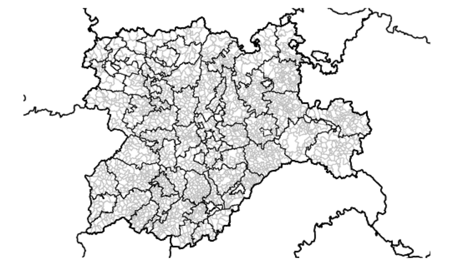
Figure 1
Castile and Leon 2248 municipalities (in grey) and 76 comarcas (in black)
Source: Own elaboration of data from www.ine.es
2.2. Fertility indexes
In this study we incorporated several fertility measures to analyse spatial patterns, using the data described in section 3.1 for the time period 1981-2018. Births are available on a yearly basis for this period; however, the continuous population register only provides yearly data at the municipal level from 1998. Thus, for population before 1998, we use estimates from the 1981 and 1991 population census and the 1986 census derived from the population register and interpolated the yearly figures using a cohort approach. The final dataset contains female midyear population counts for 7 five-year age groups, 38 calendar years from 1981 to 2018, 910 geographical areas, and three birth orders (first, second, third and above). We then compute three sets of indicators, for total and parity specific fertility levels: Age Specific Fertility Rates (ASFR), Total Fertility Rates (TFR), and Mean Age at Childbearing (MAC).
2.3. Method
In this paper we have used and tested different types of classical contiguity definitions and arbitrarily defined distances to look at the effect of neighborhood definition on spatial autocorrelation over time. In particular, we have used definitions based on boundaries and distance as shown in Table 2.
Distance band defined neighborhood relations are constructed on a pre-determined centroid distance between each i and j pair of spatial units. The number of connections for each area usually varies, and depending on the selected distance, there may be empty sets of neighbors. K-Nearest Neighbors ranks spatial units and creates sets each containing the exact same number k of closest units to i.
Boundaries based contiguity definition relies on whether spatial units share a boundary or not. The weight matrix can also be row-standardized according, and divided by the number of neighbors or alternatively variance-stabilized (Tiefelsdorf and Griffith, 1999). In this study we have implemented all aforementioned standardizations in order to evaluate their impact on spatial autocorrelation measures.
First order queen contiguity denotes a set of boundary points b of unit i, which share at least a single boundary point, whereas, first order rook denotes a set of boundary points b of unit i, which share a positive proportion of their boundary, thus having length >0.
The choice of comparing different neighborhood matrices relies upon the fact that, in spatial analysis, the selection of a particular proximity definition can substantially impact spatial autocorrelation, as will later be shown through correlogram analysis. In our study, we offer a quantifiable overview of how spatial autocorrelation varies with the neighborhood definition. Once the spatial neighbor list has been defined, we define the spatial weight matrix so that the weights for each areal item sum up to unity.
Distance and neighboring relations between different areas can be useful to understand how spatial dependence works and on "how close places need to be" in order to be related, or in other words, spatially autocorrelated. Of the various tools used in spatial econometrics to understand spatial dependence, Moran's I Index is one of the most frequently used to help quantify the global level of autocorrelation. Moran’s I is the index obtained through the product of the variable considered, y, and its spatial lag, with the cross product of y and adjusted for the spatial weights considered:
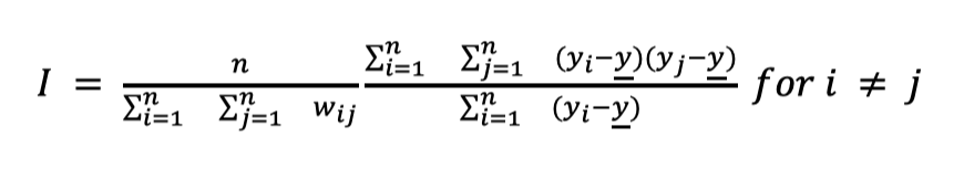
(1)
where n is the number of spatial units i and j, yi is the ith spatial unit, Importar imagen is the mean of y, and wij is the spatial weight matrix, where j represents the regions adjacent to i. Moran’s I can take on values [-1,+1], where – 1 represents strong negative autocorrelation, 0 no spatial autocorrelation and 1, strong positive autocorrelation.
This measure can be broken down into its local components in order to identify clusters of areas with variables displaying similar values, where clusters are defined as observations with similar neighbors (Anselin, 1995). The procedure is known as Local Indicators of Spatial Association (LISA), where the Local Moran’s I decomposes global Moran's I into its contributions for each location. These indicators detect clusters of either similar or dissimilar values around a given observation. The relationship between global and local indicators is quite simple, as the sum of LISAs for all observations is proportional to Moran's I. Therefore, LISAs can be interpreted both as indicators of local spatial clusters and as pinpointing outliers in global spatial patterns.
The measure for LISAs is defined as:
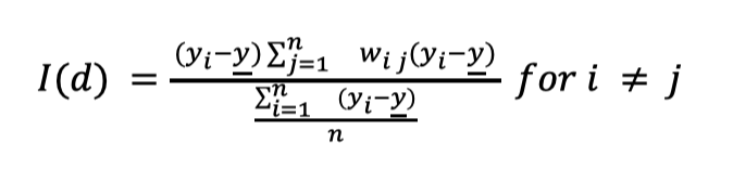
(2)
where the global mean is assumed to be an adequate representation of the variable of interest y.
In order to understand the effect of distance on spatial autocorrelation, we measure Moran’s I using the correlogram (Cliff and Ord, 1981, 1970; Goovaerts, 1997) technique for various variables at different points in time. Plotting Moran’s I over increasing distance, I(d), thus obtaining a correlogram, can be particularly insightful as it produces an easily understandable depiction of how spatial autocorrelation evolves as the distance between centroids rises. In our study, we constructed correlograms by employing the R package pgirmess (Giraudoux, 2013), which uses Sturges’ method (Sturges, 1926) to compute the optimal number of bins and uses normal approximation to test for significance:
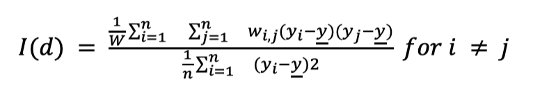
(3)
where I(d) is Moran’s I correlation coefficient as a function of distance d, yi and yj
and are the values of the variable at locations i and j, W is the sum of the values of the matrix, and N is the sample size.
We carried out this analysis first using mainland Spain, 858 areas excluding Canary and Balearic Islands, applying a correlogram analysis for all the indicators considered in this study. Since one of our main hypotheses was that spatial autocorrelation reflects the highly cultural and linguistic heterogeneity in the country, we implemented the same technique for each macro-region with at least 30 comarcas (see figure 2 and table 1 for details), to understand whether there are unique spatial autocorrelation paths, and if those paths differ across macro regions. The grouping of mainland regions with fewer than 30 units aims at maintaining historical and cultural information.
| Family | Type | Contiguity | |
| Distance Based | Distance band K-Nearest Neighbors (KNN) | 1. 5 nearest neighbors2. 10 nearest neighbors 3. 15 nearest neighbors | |
| Boundaries Based | Spatial Contiguity | 1. First Order Queen (FOQ) 2. Second Order Queen (SOQ) 3. First Order Rook (FOR) 4. Second Order Rook (SOR) | |
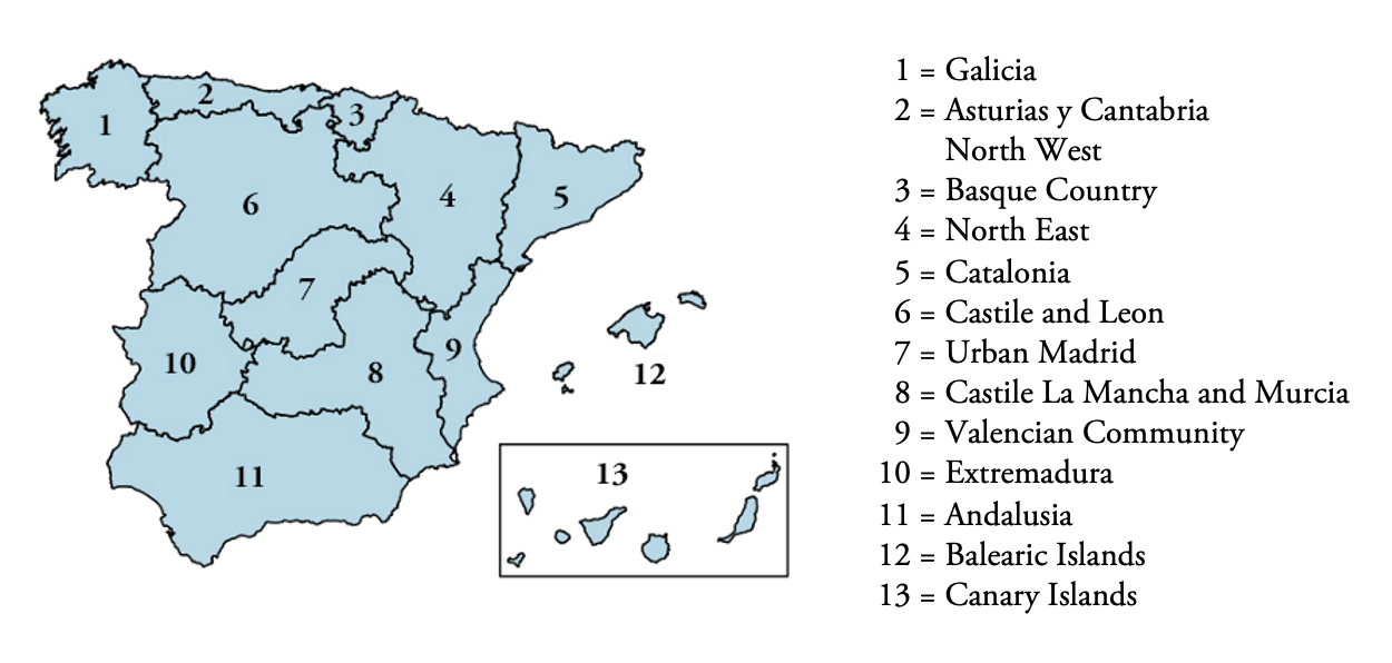
Figure 2
Subdivision of Spain into macro-regions
Source: Own elaboration of data.
3. Results
Spain is a highly diverse country, where geography plays a crucial role in defining spatial patterns of fertility. Starting from the assumption that there is fertility diversity across the country, which persists over time and that such variance is not random but rather spatially driven, we aimed to describe the divergence from national trends and analyze the dynamics of spatial patterns of fertility over time by means of spatial analysis. We have structured the results section in three parts: a description of subnational fertility over the last 38 years, a global spatial autocorrelation analysis using Moran’s I and correlogram analysis to assess the variation of spatial autocorrelation of fertility indicators with different neighboring definitions through time, and lastly employing measures of local spatial association, LISA, to assess the evolution of geographical dependency across years and to identify spatial clusters of fertility.
To facilitate the geographical reading of the results we have grouped the 910 areas into 13 macro-regions (see figure 2 and table 1), which try to preserve historical, linguistic, and cultural boundaries. This grouping of Autonomous Communities into larger regions is the definitive version of various tests, which provide the best readability of our results. We joined the province of Madrid together with Toledo and Guadalajara (Burns et al. 2009); Castile and La Mancha with Murcia, Asturias, and Cantabria (North-West); Aragon, La Rioja, and the Foral Community of Navarra (North-East).
In the analysis, we do not include any indicator for migrants’ fertility. Recent studies (Arango and Finotelli, 2009; Devolder and Bueno, 2011; Devolder and Cabré Pla, 2009; Devolder and Trevino, 2007; Recaño and Roig, 2006) have emphasized how the migrants’ influx has impacted Spanish birth rates, contributing substantially to the latest fertility recuperation. Nevertheless, given the concentration of migrants predominantly in big cities such as Barcelona and Madrid, and the lack of significance for spatial measures of migrants’ fertility, we prefer to focus our attention to the whole population without differentiating by nationality.
3.1. Descriptive
Since the mid-1970s, Spain has been quickly approaching under-replacement fertility levels, reaching its lowest-low levels (<1.3 children per woman) in 1993 (Kohler, Billari, and Ortega, 2002) with mean age at childbirth steeply increasing past 30 years old (Sobotka, 2008). Even though this decrease slightly reversed later, with childbearing postponement slowing and fertility increasing to 1.45 children per woman up until the 2008 economic crisis, which has lowered childbearing, TFR swung back up to 1.26 children per woman in 2018[2]. Such changes in childbearing have not been geographically homogeneous throughout Spain, but rather characterized by the presence of a sizable regional variability. Since 1981, the steep decline in fertility led to levels as low as 1.16 children per woman in 1996. Such decline was universal in Spain, but some areas displayed substantially different levels of fertility, ranging from 2.2 to 0.8 children per woman. Thus the decrease in fertility described by national level rates does not fully capture the geographical differences already present in 1981: a clear North-South line centered on Madrid, with Andalusia, Extremadura, Castile la Mancha, Murcia, and Valencian Community displayed high fertility, while the North (Catalonia, North-East, North-West, Basque Country and Galicia) registered below replacement fertility, with the province of Burgos (Castile and Leon), and Pontevedra (Galicia) already below 1 child per woman (Figure 3 and 5). In 1981, 10 areas out of 910 already had a mean age at childbearing slightly above 30 years old. Every year after, this number almost doubled, with the biggest jump occurring between 1993 and 1994, which saw an increase in the count of areas with a mean age at childbearing above 30 years old from 112 to 210 (Figures 4 and 5).
By the mid-1990s fertility reached a lowest-low point in Spain (<1.3), again with important differences between regions: the North of the country reaching minimal levels as early as 1993 (Asturias and Cantabria) and 1995 (Catalonia), the South seeing a slow decline in fertility until 2002 (Andalusia Castile La Mancha, Extremadura), and the Canary Islands never ceasing to have declining fertility levels (see Figure 3).
During the mid-1990s, the North of Spain was once again leader of the lowest fertility in the country and the highest mean age at childbearing, while the South kept somewhat higher levels in fertility (1.38 children per woman in Andalusia versus 0.8 in the North-West), and lower mean age at childbearing (27.1 years old in Andalusia versus 30.2 in the Basque Country), in 1997. The rapid childbearing postponement characteristic of the 1990s began slowing down (Goldstein, Sobotka, and Jasilioniene, 2009) due to the following factors helping to place fertility onto a recuperation path: tempo effects (Sobotka et al. 2012), the improvement of the labor market (Adsera, 2005), and the influx of immigrants (Roig and Castro, 2007). However, this reversal in fertility trends came to a halt in 2008, the year before the onset of the Great Recession, which saw levels of overall fertility at its highest since the mid-1980s. A very interesting feature of this transition lies in its spatial dimension, as fertility seems to undergo a profound geographical ‘redistribution’. Between 1981 and 2011, the North-South classical division of low-high fertility rotated to an East-West division, also centered on Madrid and encompassing Galicia, Castile and Leon, the North-West (Asturias and Cantabria) and Extremadura as low-fertility areas (Gil-Alonso, 1997; 2000), whereas big cities and extended urban areas reveal the (relatively) highest fertility (Basque Country, Catalonia, Murcia, Sevilla, and Urban Madrid) as highlighted by Bayona-i-Carrasco et al. (2016). Such East-West divide seems to persist also during the economic recession, with relative high fertility concentrating in big cities and on the East coast.
To assess the spatial dimension of the recent fertility evolution and whether such transformations imply a spatial dimension rather than a random pattern, we implemented several steps. First, we applied Moran’s I index to test the presence of underlying non-random spatial autocorrelation over time. Second, our correlogram analysis helped determine the spatial scale and its significance for all the areas and for each macro-region. Lastly, our local analysis of spatial clusters provided a visual interpretation of fertility variation through our timeframe locating high and low fertility clusters and their evolution over time.
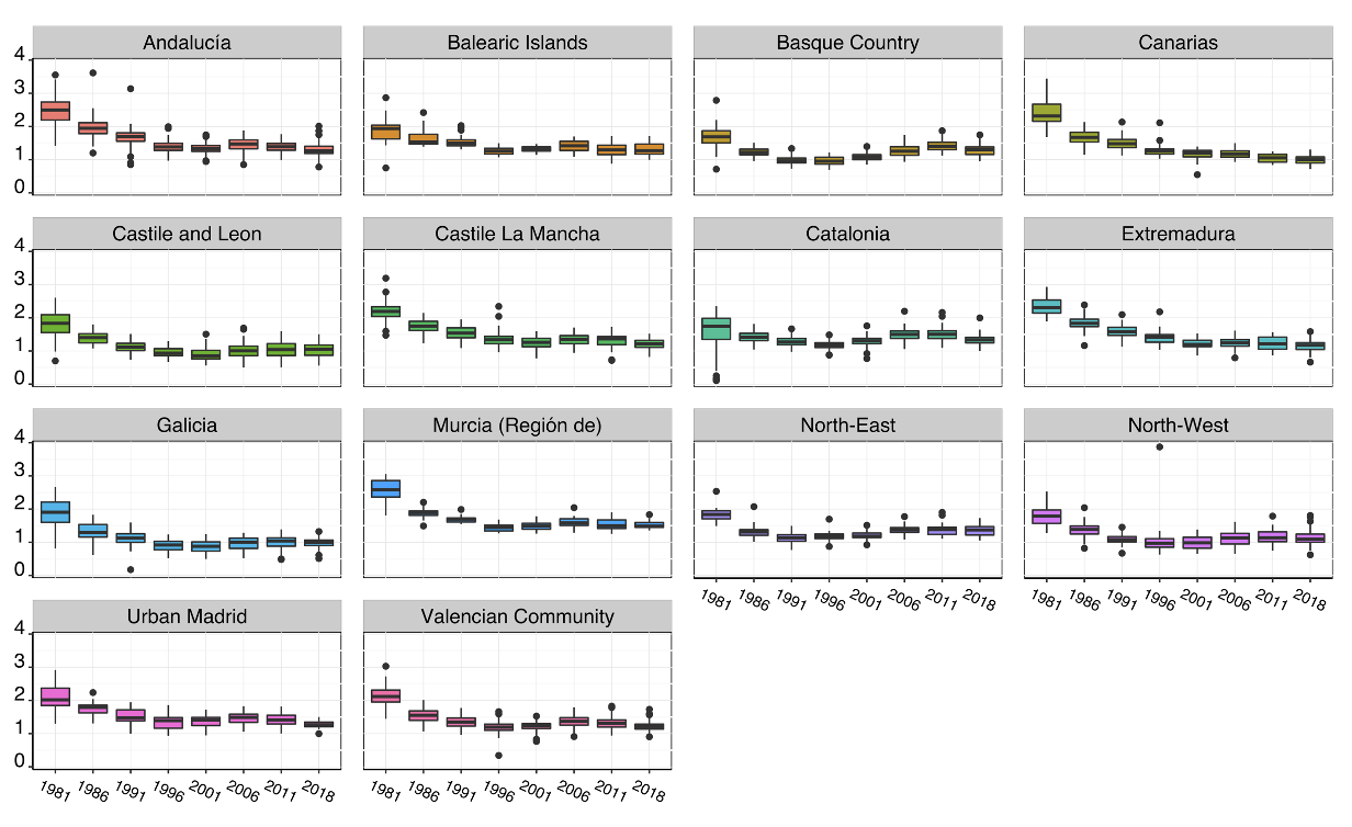
Figure 3
Boxplot for total fertility rate between for selected years by big regions
Source: Own elaboration of data, excluding Ceuta and Melilla. Source: INE https://www.ine.es/dynt3/inebase/es/index.htm?padre=2043&capsel=2047
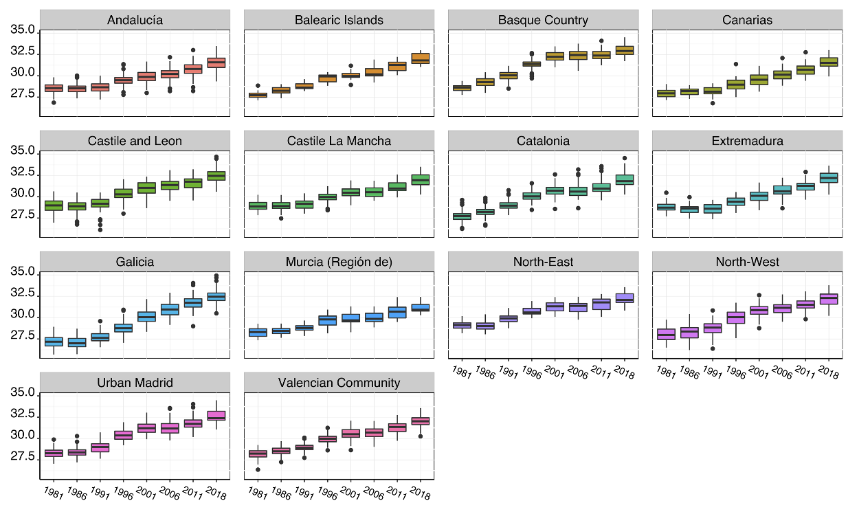
Figure 4
Boxplot for mean age at childbearing between 1981 and 2018 by big regions
Source: Own elaboration of data, excluding Ceuta and Melilla. Source: INE https://www.ine.es/dynt3/inebase/es/index.htm?padre=2043&capsel=2047.
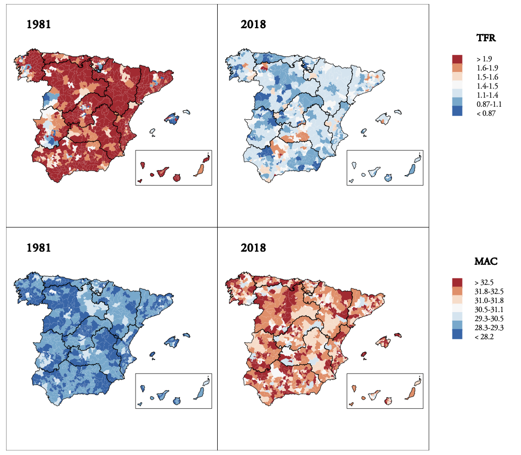
Figure 5
Total fertility rate and mean age at childbearing for years 1981 and 2018
Source: Own elaboration of data, excluding Ceuta and Melilla. Source: Vital Statistics Microdata 1979-2018; Census Microdata 1981, 1991, 2001 and 2011 and Population Register Microdata 1986 and annual statistics 1998-2018, INE.
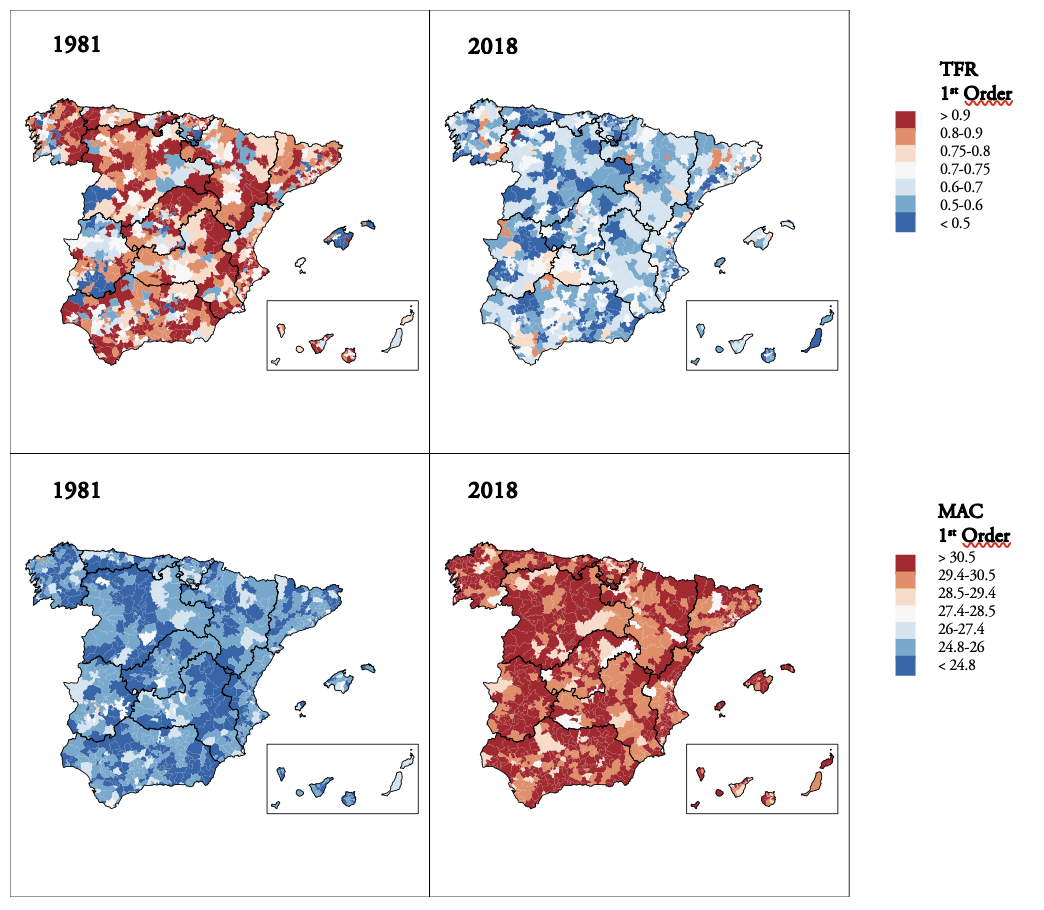
Figure 6
Total fertility rate and mean age at childbearing for the first birth order in 1981, 1997 and 2018
Source: Own elaboration of data, excluding Ceuta and Melilla. Source: Vital Statistics Microdata 1979-2018; Census Microdata 1981, 1991, 2001 and 2011 and Population Register Microdata 1986 and annual statistics 1998-2018, INE.
3.2.1. Global Moran’s I
Moran’s I quantifies the global level of autocorrelation and discerns whether the process under study is random or statistically significant, for a selected variable given a certain neighborhood matrix specification. The selection process is not a trivial issue and can substantially impact the results as it reflects the intensity of a geographical relationship between areas, changing the total number of neighbors. Therefore, in this study we applied Moran’s I test for all variables for the considered period (1981-2018) comparing results for various neighborhood specifications using different contiguity definitions and deliberately chosen distances.
The neighborhood type that captures spatial autocorrelation the best is first order rook contiguity, which has the advantage to overcome issues derived from using irregular polygons maps with varying surface areas and distances between centroids, while focusing on shared borders. This preliminary analysis is important as it demonstrates how every geographical structure requires a different, if not at the very least, a carefully chosen neighbors definition.
Moran’s I is positive and statistically significant (pvalue0.05) for all variables and for all neighborhood specifications throughout the years, suggesting that in this study there is spatial autocorrelation and the nearby areas tend to display similar fertility behaviors. TFR (Figure 7) shows a positive and statistically significant value for all birth orders over the whole considered time frame, and first order rook contiguity exhibits the highest spatial autocorrelation pattern. This outcome implies that in this study, fertility is a “small scale” phenomenon, with spatial autocorrelation decreasing with increasing lags or distance.
Moran’s I measured for TFR does not keep constant throughout the years, with fluctuating trends for all variables. For instance, Moran’s I measured for TFR at third birth order decreases by 35% in 38 years, from 0.75 to 0.5. This decrease may suggest that the occurrence of third births is getting less dependent on spatial structures, meaning that over time neighboring areas decrease their similarity. On the other hand, TFR for second birth order increases, emphasizing the bigger importance of space and location for the variable, thus the tendency to cluster together for similar values increases. First birth order fertility presents a zigzagging pattern. It is interesting to notice that the year of the minimum 1998, (1.14 children per woman) and of the maximum 2008, (1.45 children per woman) are those of fertility contraction and increase respectively.[3] This last finding is of importance and one possible explanation could be that periods of increased fertility and of economic wellbeing lead to a spatial autocorrelation increase and more prominent role of geography in determining fertility clusters, while during economic recessions fertility behavior becomes more dependent on factors other than space.
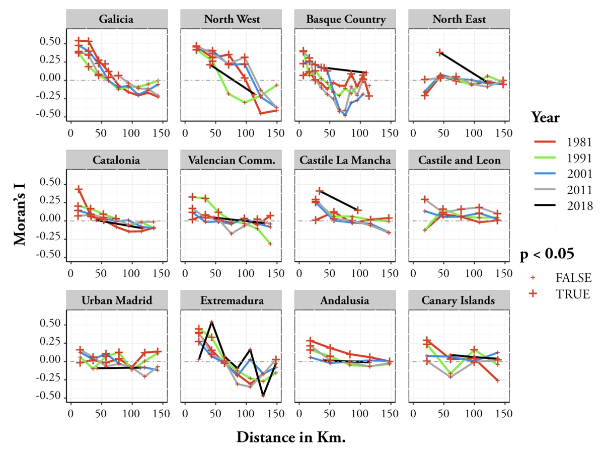
Figure 7
Correlogram plot for TFR. Regional view
Source: Own elaboration of data, excluding Ceuta and Melilla.
3.2.2. Correlogram Analysis
The advantage of contiguity-based definitions, ignoring areas specific dimensions and distances between centroids, is also its flaw Nevertheless, arbitrarily setting a distance may preclude finding important scale patterns and overlook distance dynamics. Given that spatial autocorrelation is highly scale-dependent, we implement correlogram analysis to examine patterns of spatial autocorrelation at increasing distance lags for Spain mainland and macro-regions. This method makes use of R package pgirmess (Giraudoux, 2013) and allows for computing Moran's I coefficient on an optimal number of distance classes obtained through Sturges (1929) method from a set of spatial coordinates.
The correlograms in Figure 7 display on the x-axis the centroid distance in km and on the y-axis Moran's I value, ranging from 0.5, clustering of similar values, to -0.5, indicating dispersion. To investigate whether the effect of spatial autocorrelation can be attributed to specific regional patterns, we divide the national territory into 13 macro-regions to maintain a minimum number of 30 comarcas per region to ensure Moran’s I statistical validity (see figure 2 and table 1) and compare the correlograms across years using total fertility. The first distance class (27.4 km) registers the highest positive and statistically significant spatial autocorrelation, a rather short distance, which may hint at a small-scale clustering of fertility. This distance captures the highest spatial autocorrelation of all distance bands, although with values lower than contiguity-based definitions. This result suggests the importance of testing for different neighborhood definitions carefully and not arbitrarily, as similar distance bands definitions, 20 km and 27.4 km, capture spatial autocorrelation differently. Moran's I remains significant and positive up to high distances (close to 400km) surmising that the spatial effect of fertility for distance based neighbors is a small-scale phenomenon across regions, retaining important influence at larger bounds too. Distance classes vary substantially due to each region-specific feature, the first distance class for instance ranges from 6 km for Basque Country to 22km for the Canary Islands. Figure 7 reveals distinctive paths of spatial dependency for Galicia, Catalonia, Castile Leon, Castile La Mancha, and Andalusia, reflecting a general homogeneous and decreasing effect of distance. This particularly important finding pinpoints the spatial distinctiveness of regions, such as Catalonia and Galicia, which have historically displayed not only uniqueness in socio-cultural characteristics but also in fertility behavior.
The implementation of global measures of spatial autocorrelation focuses mainly on the neighboring definition for one important reason: spatial autocorrelation is highly scale-dependent and the choice of neighborhood can deeply impact not only the magnitude of spatial autocorrelation measures, such as Moran’s I, but also its significance. Furthermore, choosing a neighborhood matrix without looking at distance scale effect, solely based on Moran’s I magnitude and significance, may also preclude from uncovering small-scale patterns that can be easily identified through correlogram analysis, as demonstrated in the following section.
3.3. Local Indicators of Spatial Association
The last part of the analysis involves the clusterization of the considered variables by means of local indicators of spatial association, LISA, which decompose the global indicator, in this case Moran’s I, into its local equivalent (Anselin, 1995). LISA have the advantage of providing a measure of spatial dependence at local level for each area, making it possible to plot the results on a map obtaining a representation of spatial association (Anselin, 1995). Thus, LISA maps provide a measure for spatial autocorrelation for each individual location, grouping similar values around a specific observation into four groups, high-high (HH in red), high-low (HL in pink), low-high (LH in light blue), low-low (LL in blue) classified by the type of spatial autocorrelation.
In this study, we applied LISA to test whether there are significant clusters of fertility in Spain and to follow their evolution over time to understand how spatial relationships have changed over the last three decades.
LISA maps offer a direct glimpse of how geographical diversity in fertility trends has evolved since 1981. As observed in section 3.1, the North-South divide for fertility is quite clear also through LISA maps (Figures 8 and 9), with the North of Spain concentrating LL LISA clusters, while the Center-South, especially Extremadura, Andalusia, and Castile La Mancha, display HH LISA clusters. This division endures through the 1990s but shifts during the following decade, with the North and West regions of the country (Galicia, North-West, and Castile and Leon) being the hot-spot for low fertility, while high fertility clusters concentrate around big urban centers like Barcelona, Madrid, Basque Country, Murcia, and Sevilla. Mean age at first birth and its progressive increase has been one of the driving forces behind the recent fertility transformation of Spain.
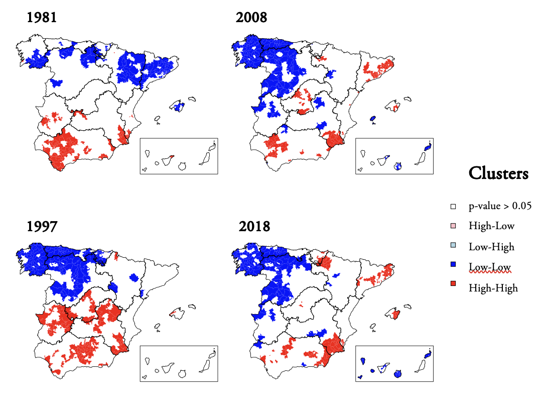
Figure 8
LISA maps for total fertility rate. Years 1981, 1997, 2008, and 2018. First Order Rook Contiguity
Source: Own elaboration of data, excluding Ceuta and Melilla.
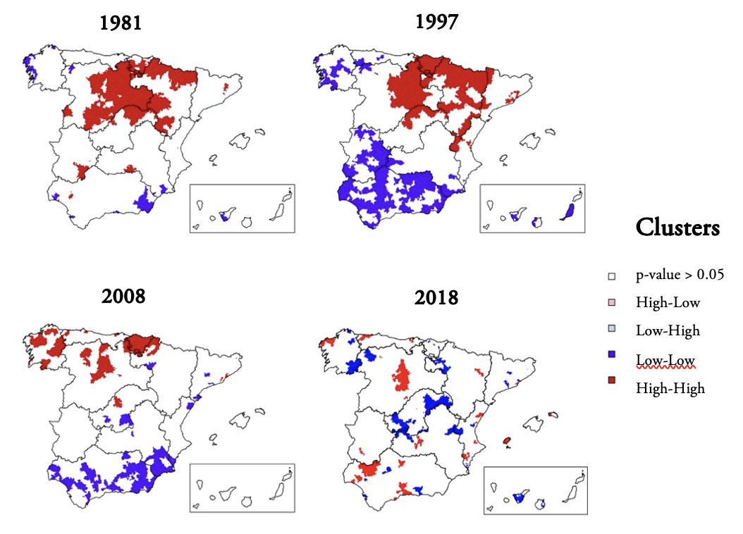
Figure 9
LISA maps for mean age at first birth. Years 1981, 1997, 2008, and 2018. First Order Rook Contiguity
Source: Own elaboration of data, excluding Ceuta and Melilla.
3.4. Exploring the determinants of change
We introduce a spatial regression model to explore the relationship between fertility and socio-economic covariates. The spatial lag model assumes that dependencies exist directly among the levels of the dependent variable and its neighboring ‘lagged’ locations. The reason for including a spatial lag into the regression model lies in the assumption that in a regular ordinary least square regression, OLS, observations should be independent of each other. This assumption is clearly violated in the presence of spatial auto-correlation, hence coefficient estimates would be biased.
We define the spatial lag model as:
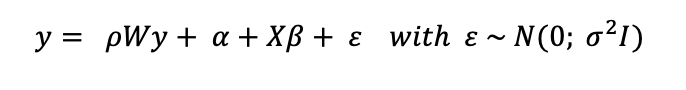
(4)
The spatial components are represented by , where is the spatial-autoregressive coefficient, W is the row-standardized n x n spatial weight matrix, and y is a n x 1 vector of observations of the dependent variable of n=910 comarcas. X is a n x k matrix of observations of k independent variables, is a vector of error terms assumed to have autocorrelation, and is a vector of k x 1 regression coefficients. We select rook neighbourhood definition following section 3.2 results on spatial autocorrelation.
We check the set of covariates for collinearity through a variance inflation factor (VIF), which must score below 4.0 (Fox and Weisberg, 2018). The appropriateness of the spatial lag has been assessed using Anselin (1988) Lagrange Multiplier test, which needs to be non-significant to confirm the absence of spatial autocorrelation (and thus bias) in the model. We apply this model to explain fertility change for each year where explanatory variables are available and utilize as dependent variable the average of fertility two years prior and after for a total of four time points (1981, 1991, 2001, 2011), whose choice is dictated mainly by the availability of covariates with the maximum spatial disaggregation. The model results include the following evaluation metrics: Likelihood ratio test (LR test), which tests whether the spatial model appropriateness; the Lagrange multiplier test (LM test) for residual autocorrelation; the AIC for the selected model, and the OLS counterpart.
3.4.1. Results of the spatial lag model
Tables 3 presents the results for the spatial lag model and its AIC measurements. The spatial lag model is the best approach as LR test value appears to be positive and statistically significant as well as AIC scores for the spatial lag model is smaller than its OLS counterpart. The indexes included in Table 3 (lower part) suggest that our lag model is the right choice and successfully removes the bias arising from spatial correlation. All rho(s) are positive, significant, and substantially lower than the Moran’s I reported in Table 2, signifying the ability of the spatial lag model to capture the bias arising from spatial autocorrelation in the dependent variable. Rho(s) represents an extra spatial covariate that summarises the clustering of fertility: when fertility rises in an area, other neighboring areas will follow even after controlling for all the other covariates. The LM test value for model residuals confirms the appropriateness of the spatial lag model. Overall, all the socio-economic covariates included in the model contribute to explain the changes in fertility and help depicting a clearer picture of what factors play a crucial part. The covariates can be divided in three main categories: variables associated with family formation (i.e., age at first birth, births outside of wedlock), with labor market (i.e., female activity rate), and with migration (i.e. presence of Latin American women).
Since 1981, the fast transformation of the family into more secular forms is mirrored by the results reported in Table 3. Indeed, fertility shifted from being negatively impacted by the presence of births outside of wedlock and the proportion of married women, as marriage was the universal form of family formation and births outside of wedlock were a rare event (Rutigliano & Andersen, 2018). Marriage is increasingly tied to childbearing, shifting from being the official start of cohabitation and leaving the parental home to family formation. Similarly, births outside of wedlock shift from being rare in the 1980s and 1990s and having a negative impact on total fertility, to becoming statistically non-significant in 2011. Mean age at first birth is the only explanatory variable that is negative throughout the four time periods, although it declines in magnitude, possibly parallel to a universal fertility decrease and later childbearing.
It is interesting to observe that another covariate that keeps a constant and significant effect is the proportion of working age population with a fixed contract. Indeed, job stability has often been identified as one key factor that positively influences total fertility (Adsera, 2004). Labor market related covariates (Table 3: rows 6-9) can be seen as indicators of a society shifting away from the male breadwinner model (high positive impact of male activity rate in 1981 on total fertility), to a labor market where women’s presence in specialized jobs (higher education access by women) is increasingly more and more common and having a positive impact on total fertility (Adsera, 2004; Requena & Salazar, 2014). Female participation switches from negative in 1981 to positive in 2001, year close to economic expansion in Spain before the 2008 economic recession, which led to a general contraction of fertility rates in all countries affected (Sobotka, Skirbekk, & Philipov, 2011).
| 1981 | 1991 | 2001 | 2011 | |||||
| (Intercept) | 2.74 | *** | 0.93 | * | -0.51 | *** | -0.40 | |
| Mean age at first birth | -0.14 | *** | -0.08 | *** | -0.01 | * | -0.03 | *** |
| High education female | 1.11 | ‘ | 1.46 | *** | 0.23 | *** | 0.95 | *** |
| % of married women | -1.60 | *** | 0.62 | *** | 1.08 | *** | 1.89 | *** |
| % out of wedlock births | -1.65 | *** | -0.92 | *** | 0.32 | *** | 0.06 | |
| Male activity rate | 2.09 | *** | 1.18 | *** | 0.22 | *** | 0.28 | ‘ |
| Female activity rate | -0.96 | *** | 0.07 | 0.14 | *** | 0.14 | ||
| % Employed fixed contract | 0.60 | *** | 0.71 | *** | 0.54 | *** | 0.48 | *** |
| % Employed in tertiary | 0.83 | *** | 0.75 | *** | -0.004 | -0.14 | ‘ | |
| Area2 | 0.02 | ** | -0.03 | *** | 0.001 | 0.03 | *** | |
| % Latin American women | -0.05 | 0.67 | *** | |||||
| % African women | 2.90 | *** | 2.80 | *** | ||||
| Rho:LR test value: | 0.2545.32*** | 0.26 48.56*** | 0.25 61.81*** | 0.21 43.42*** | ||||
| AIC:AIC for ols: | 227.62 270.93 | -440.19 -393.64 | -2065.5 -2005.7 | -947.41 -906 | ||||
| LM test value:p-value: | 4.37 0.037’ | 1.26 0.261 | 2.76 0.097 | 0.31 0.58 | ||||
Years 2001 and 2011 include an extra set of covariates that measure migrant women’s presence, as migration to Spain began in the late 1990s early 2000s and its effect was still negligible in 1991. The presence of women of childbearing age born in African countries is positive and significative for both periods included, signifying that comarcas in which their presence is higher also register higher total fertility. This finding is in line with a corpus of research that attests a much higher fertility of African migrants, with respect to Spanish born women (Stonawski, Potančoková, & Skirbekk, 2016; Vila & Martin, 2007). However, Latin American women’s effect is not so straightforward, and although significant and positive for 2011, it is smaller than that of African women. Indeed, Latin American women’s transition to first birth happens earlier although overall, they exhibit fertility schedules very similar to those of Spanish born women (Devolder, & Bueno, 2011; Gonzalez-Ferrer et al., 2017).
4. Discussion
In this article, we studied the presence of spatial autocorrelation in childbearing behavior across 910 Spanish geographical units over a 38-year period (1981-2018). Spain is a country with outstanding diversity, with linguistic and cultural identities, which often translate “demographically” into heterogeneous fertility trends, substantially varying from region to region and province to province. Our main contribution has been in employing data at a smaller geographical scale for an extended period that covers the most recent decades. We have highlighted important divergences in childbearing trends across the country that could not be evinced from national, regional, or even provincial data. Employing spatial analysis tools such as Moran’s I, correlogram analysis, LISA maps, and spatial regression have proven the existence of positive and significant clustering of areas with similar values. Indeed, our main hypothesis that there is spatial autocorrelation in fertility behavior for all variables throughout the considered period is supported by the results, both at a global and local scale.
Moran’s I results for all the considered variables indicate that spatial autocorrelation is present throughout the considered time frame and does not decrease over time, but rather fluctuates, seemingly decreasing during times of fertility decline, such as in the mid 1990s, and increasing at times of fertility expansion, as in the 2000s. This variation, however, does not see spatial autocorrelation disappear, but remains positive and high throughout the decades considered. This finding is of importance as between 1981 and 2018, the difference in childbearing indices among the various areas seems to decrease, hinting at a reduction of the spatial divergence and at a likely reduction in spatial autocorrelation as well due to convergence in trends. Even though graphic or cartographic representation of fertility trends may be helpful, the sole heuristic approach is not enough to identify and assess fertility trends non-randomness. Indeed, further analysis using spatial techniques proves the possibility of a decrease in spatial autocorrelation wrong, as spatial variation is present throughout the considered timeframe and does not decrease over time.
The comparison between contiguity and distance-based weights matrices suggests that the choice of a specific neighborhood definition is not a trivial process. In this study, first rook contiguity proves to be the specification capturing the highest spatial autocorrelation, thus ignoring distances in a map where areas surface and distances between centroids can vary substantially. The employment of correlogram analysis also helps in providing a scale to spatial autocorrelation: highest at very small distances, positive and significant at large distances, thus spatial clustering of fertility can be expected to be a small area phenomenon (first order neighbors) with the ability to encompass large areas. Moreover, the application of correlogram analysis to single macro-regions highlights significant and positive spatial autocorrelation and autocorrelation patterns that persist in time (as for Galicia and Catalonia). This finding is particularly important as it stresses the role of regional autonomies not only with specific cultural and linguistic identities but also with a documented history of distinct childbearing patterns (Cabré Pla, 1999; Cabré Pla and Pujadas Rúbies 1989; Devolder & Cabré Pla, 2009; Leasure, 1963; Livi-Bacci, 1968a, 1968b).
The advantage of employing spatial analysis is not only to globally assess the presence of spatial autocorrelation, that similar values tend to cluster together, but also to identify such clusters. Indeed, LISA cluster analysis helps to depict the shift in the geographical distribution of fertility over the country. The last three decades have seen a profound transformation in fertility trends across the Iberian country with a sharp decrease in overall fertility and delay of childbearing, but with substantial differences in space that do not match provincial boundaries. Cluster analysis shows not only that spatial autocorrelation does not disappear, but also that over time clusters change. The classic North-South division ceases to exist leaving room for high fertility clusters located in big cities such as Madrid, and Barcelona (see i.e., Bayona-i-Carrasco et al., 2016; Lopez-Villanueva et al., 2014; Pujadas Rúbies et al., 2013) and the North-West to emerge as the focal point for low fertility (Gil-Alonso, 2000).
Spatial regression is the appropriate method to explain changes in fertility as it provides results unbiased by spatial correlation. It also gives insights on which factors had a substantial role in shaping fertility. Indeed, the biggest changes throughout time that impacted Spain can be identified in the variables considered in our model: family formation, labor market and migration. Marriage has become an indicator for family-oriented values (Adsera, 2006) and is the strongest predictor of higher fertility after African migrants’ presence. Persistent shocks to the economy still negatively impact fertility. Among all labor market indicators, job stability (and proportion having a fixed contract) holds a constant positive effect throughout almost four decades. Moreover, female participation to the labor force has shifted sign and has become a positive influence on overall fertility, signifying that areas with higher female activity rate also show higher fertility rates, thus furthering the positive relationship between fertility and economic conditions.
The subnational perspective on fertility provides the chance to examine how socio-economic determinants affect fertility dynamics, but it can also contribute to deepen our understanding of how fertility clusters evolve through time. Further research is clearly needed, especially employing data that can offer detailed age groups, both for women and men, to better focus the analysis on individuals of childbearing age.
Availability of data and materials
The data sources utilized in this study are: Vital Statistics Microdata 1979-2018; Census Microdata 1981, 1991, 2001 and 2011, and Population Register Microdata 1986 and Padrón Continuo database 1998-2018 provides population data by calendar year.
The data implemented in this study come from custom extractions of data from the Spanish National Institute, INE:
(1) Microdatos del Censo de 1981, Padrón de 1986, Censo de 1991 y Padrón Continuo for all years between 1998 and 2018;
(2) Microdatos del Movimiento Natural de la Población for years 1979-2018 for births by age of mother and by municipality.
Elaborated data and R code can be made available by contacting the authors.
Acknowledgments
Discussions with colleagues on various occasions have contributed to this study.
References
Adsera, A. (2004). Changing fertility rates in developed countries. The impact of labor market institutions. Journal of population economics, 17(1), 17-43.
Adsera, A. (2005). Vanishing children: from high unemployment to low fertility in developed countries. American Economic Review, 95(2), 189–193.
Adsera, A. (2006). Marital fertility and religion in Spain, 1985 and 1999. Population Studies, 60(2), 205-221.
Alonso, F. G. (1997). Las diferencias territoriales en el descenso de la fecundidad en España. Aproximación a su estudio a partir de datos censales sobre fecundidad retrospectiva. Boletín de la Asociación de Demografía Histórica, 15(2), 0013-54.
Alonso, F. G. (2000). El descenso de la fecundidad en el nordeste peninsular. Documents d'Análisi Geográfica, 36, 111–132.
Anderson, B. A. (1986). Regional and cultural factors in the decline of marital fertility in Western Europe. In A. J. Coale and S. C. Watkins (Eds.), The Decline of Fertility in Europe (pp. 293–313). Princeton University Press.
Anselin, L. (1995). Local indicators of spatial association-LISA. Geographical Analysis, 27(2), 93–115.
Arango, J., & Finotelli, C. (2009). Past and future challenges of a Southern European migration regime: the Spanish case. IDEA Working Papers, 8, 443-457.
Arpino, B., & Tavares, L. P. (2013). Fertility and values in Italy and Spain: a look at regional differences within the European context. Population Review, 52(1).
Basten, S., Huinink, J., & Klüsener, S. (2011). Spatial variation of sub-national fertility trends in Austria, Germany and Switzerland. Comparative Population Studies, 36(2-3).
Bayona-i-Carrasco, J., Rubiales, M., Gil-Alonso, F., & Pujadas, I. (2016). Causas de las desigualdades territoriales en la fecundidad: un estudio a escala metropolitana en el área barcelonesa. Revista de Geografía Norte Grande, 65, 39-63.
Bocquet-Appel, J. P., & Jakobi, L. (1998). Evidence for a spatial diffusion of contraception at the onset of the fertility transition in Victorian Britain. Population: An English Selection, 181–204.
Brown, J. C., & Guinnane, T. W. (2002). Fertility transition in a rural, catholic population: Bavaria, 1880-1910. Population Studies, 56(1), 35–49.
Burns, M. C., Cladera, J. R., Bergadà, M. M., & Seguí, M. U. (2009). El sistema metropolitano de la macrorregión de Madrid. Urban, 14, 72-79.
Cabré, A., & Pujadas, I. (1989). La población: inmigració i explosió demogràfica. Història económica de la Catalunya contemporània s. XX Població, agricultura i energía, 11-128.
Cabré, A. M. (1999). El sistema catalá de reproducció, (Vol. 35). Barcelona, Proa.
Cliff, A. D., & Ord, J. K. (1981). Spatial processes, models and applications. Pion, London.
Cliff, A. D., & Ord, J. K. (1970). Spatial autocorrelation: A review of existing and new measures with applications. Economic Geography, 46(sup1), 269-292.
Coale, A. J., & Watkins, S. C. (1986). The decline of fertility in Europe: the revised proceedings of a conference on the Princeton European Fertility Project. Princeton: Princeton University Press.
Delgado Pérez, M. (2009). La fecundidad de las provincias españolas en perspectiva histórica. Estudios Geográficos, 70(267), 387–442.
Devolder, D., & Bueno, X. (2011). Interacciones entre fecundidad y migración. Un estudio de las personas nacidas en el extranjero y residentes en Cataluña en 2007. Documents d'anàlisi geogràfica, 57(3), 441-467.
Devolder, D., & Cabré, A. (2009). Factores de la evolución de la fecundidad en España en los últimos 30 Años. Panorama Social, 10, 23–39.
Devolder, D., Nicolau, R. N., & Panareda, E. (2006). La fecundidad de las generaciones españolas nacidas en la primera mitad del siglo XX: un estudio a escala provincial. Revista De Demografía Histórica, 24(1), 57–90.
Devolder, D., & Treviño, R. (2007). Efectos de la inmigración extranjera sobre la evolución de la natalidad y de la fecundidad en España. Barcelona: Centre d’Estudis Demogràfics, Papers de Demografia, 321.
Fernández Cordón, J. A. (1986). Análisis longitudinal de la fecundidad en España. Tendencias demográficas y planificación económica. Madrid: Ministerio de Economía y Hacienda, 49-75.
Gil-Alonso, F. G. (1997). Las diferencias territoriales en el descenso de la fecundidad en España. Aproximación a su estudio a partir de datos censales sobre fecundidad retrospectiva. Boletín de la Asociación de Demografía Histórica, 15(2), 13-54.
Gil-Alonso, F. G. (2000). El descenso de la fecundidad en el nordeste peninsular. Documents d'Análisi Geográfica, 36, 111–132.
Giraudoux, P. (2013). pgirmess: data analysis in ecology. R package version 1.5.8.
Goldstein, J. R., Sobotka, T., & Jasilioniene, A. (2009). The end of “lowest-low” fertility? Population and Development Review, 35(4), 663–699.
González-Ferrer, A., Castro-Martín, T., Kraus, E. K., & Eremenko, T. (2017). Childbearing patterns among immigrant women and their daughters in Spain: Over-adaptation or structural constraints? Demographic Research, 37, 599-634.
Goovaerts, P. (1997). Geostatistics for natural resources evaluation (p. 489). Oxford University Press.
Herrador, M., & Alvarez, M. A. (2007). Trabajos experimentales para la producción de datos EPA comarcales. https://www.ine.es/docutrab/epa_comarcas/epa_comarcas.pdf Instituto Nacional de Estadística.
Klüsener, H.P., Devos, I., Ekamper, P., Gregory, I., Gruber, S., Martí-Henneberg, J., van Poppel, F., da Silveira, L., & Solli, A. (2014). Spatial inequalities in infant survival at an early stage of the longevity revolution: A panEuropean view across 5000+ regions and localities in 1910. Demographic Research, 30, 1849-1864.
Kohler, H. P., Billari, F. C., & Ortega, J. A. (2002). The emergence of lowest‐low fertility in Europe during the 1990s. Population and Development Review, 28(4), 641–680.
Leasure, J. W. (1963). Factors involved in the decline of fertility in Spain 1900-1950. Population Studies, 16 (3), 271–285.
Livi-Bacci, M. (1968). Fertility and nuptiality changes in Spain from the late 18th to the early 20th Century: Part I. Population Studies, 22(1), 83–102.
Livi-Bacci, M. (1968). Fertility and nuptiality changes in Spain from the late 18th to the early 20th century: Part 2. Population Studies, 22(2), 211–234.
López-Villanueva, C., Gil-Alonso, F., Bayona, J., & Thiers, J. (2014). Efectes de la suburbanització i la immigració internacional en l'evolució recent de la fecunditat a Catalunya: Un estudi territorial a escala local. Documents d’Analisi Geogràfica, 60(3).
Moran, P. A. P. (1950). Notes on continuous stochastic phenomena. Biometrika, 37, 17–23.
Pujadas, I., Bayona-i-Carrasco, J., Gil-Alonso, F., & López, C. (2013). Pautas territoriales de la fecundidad en la Región Matropolitana de Barcelona (1986-2010). Estudios Geografícos, LXXIV(275), 585-609.
Recaño, J., & Roig, M. (2006). The internal migration of foreigners in Spain. Centre d’Estudis Demogràfics.
Requena, M., & Salazar, L. (2014). Education, marriage, and fertility: The Spanish case. Journal of Family History, 39(3), 283-302.
Roig, M., & Castro, T. (2007). Childbearing patterns of foreign women in a new immigration country: the case of Spain. Population (English Edition), 62(3), 351–379.
Rutigliano, R., & Esping-Andersen, G. (2018). Partnership choice and childbearing in Norway and Spain. European Journal of Population, 34(3), 367-386.
Sáez, A. (1979). La fécondité en Espagne depuis le début du siècle. Population (French edition), 1007-1021.
Schmertmann, C.P., Potter, J.E., & Cavenaghi, S.M. (2007). Exploratory analysis of spatial patterns in Brazil’s fertility transition. Population Research and Policy Review, 27(1), 1-15.
Sharlin, A. (1986). Urban-rural differences in fertility in europe during the demographic transition. In A. J. Coale and S. C. Watkins (Eds.), The Decline of Fertility in Europe (pp. 201–233). Princeton University Press.
Sobotka, T. (2008). Overview chapter 6: The diverse faces of the Second Demographic Transition in Europe. Demographic Research, 19(8), 171–224.
Sobotka, T., Skirbekk, V., & Philipov, D. (2011). Economic recession and fertility in the developed world. Population and development review, 37(2), 267-306.
Sobotka, T., Zeman, K., Lesthaeghe, R., Frejka, T., & Neels, K. (2012). Postponement and recuperation in cohort fertility: Austria, Germany and Switzerland in a European context. Comparative Population Studies - Zeitschrift Für Bevölkerungswissenschaft, 36(2-3), 417–452.
Stonawski, M., Potančoková, M., & Skirbekk, V. (2016). Fertility patterns of native and migrant Muslims in Europe. Population, space and place, 22(6), 552-567.
Sturges, H. (1926). The choice of a class interval. Journal of the American Statistical Association, 21(153), 65–66.
Tiefelsdorf, M., & Griffith D. A. (1999). A variance stabilizing coding scheme for spatial link matrices. Environment Planning A, 31(1), 165–180.
Tobler, W. (1970). A computer movie simulating urban growth in the Detroit region. Economic Geography, 46(2), 234–240.
Vila, M. R., & Martín, T. C. (2007). Childbearing patterns of foreign women in a new immigration country. Population, 62(3), 351-379.
Vitali, A., Aassve, A., & Lappegard, T. (2015). Diffusion of childbearing within cohabitation. Demography, 52(2), 355–377.
Información adicional
JEL Classification:: J11; C31
Funding: We would like to acknowledge financial support from the Ministerio de Economía y Competitividad. Programa Estatal de Investigación, Desarrollo e Innovación Orientada a los Retos de la Sociedad. Plan Estatal de Investigación Científica y Técnica y de Innovación 2013-2016 (CSO2013-45358-R: Movilidad geográfica y acceso a la vivienda. España en perspectiva internacional), and Comportamientos demográficos y estrategias residenciales: apuntes para el desarrollo de nuevas políticas sociales (CSO2016-79142-R).