Articles
The influence of agglomeration on growth: A study of Argentina
The influence of agglomeration on growth: A study of Argentina
Investigaciones Regionales - Journal of Regional Research, núm. 51, pp. 33-61, 2021
Asociación Española de Ciencia Regional

Esta obra está bajo una Licencia Creative Commons Atribución-NoComercial 4.0 Internacional.
Recepción: 08 Julio 2019
Aprobación: 08 Octubre 2021
Abstract: This paper analyses the influence of agglomeration on economic growth in the Argentinian provinces for the period 1981–2007 using fixed effects and GMM estimation for panel data. The choice of the estimation approach is crucial. After controlling for potential simultaneity bias, there is evidence of a link between agglomeration and growth in the Argentinian provinces, suggesting that the Williamson hypothesis is in place.
Keywords: Regional growth, agglomeration, Williamson hypothesis, Argentina.
Resumen: El trabajo analiza el efecto de la aglomeración sobre el crecimiento económico en las provincias argentinas para el período 1981-2007 utilizando estimaciones de efectos fijos y de GMM dinámico. La elección del enfoque de estimación es crucial. La utilización de GMM para reducir el sesgo de simultaneidad permite observar una relación entre aglomeración y crecimiento en las provincias argentinas que sugiere que la Hipótesis de Williamson está vigente.
Palabras clave: Crecimiento regional, aglomeración, hipótesis de Williamson, Argentina.
Introduction
This paper analyses the link between growth and urbanization, focusing on the perspective proposed by Duranton (2014),[1] who argued that growth is affected by urbanization in opposition to the traditional – and repeatedly documented – causation from economic growth to increased urbanization (Henderson,
The study of the effect of agglomeration on growth is relevant in itself but especially for Argentina since a major challenge for developing countries is to reinforce the role of their urban systems as drivers of economic growth. Argentina is a particularly interesting case as it consists of provinces with important differences in terms of natural resources, population, skills, and even political issues. These are critical when analysing growth.[2]
The research responds to two spatial organization principles that are closely linked: (a) the principle of agglomeration or synergy, studied by theorists such as Alfred Marshall, Alfred Weber, William Alonso, and Raymond Vernon, among many others (even Max Weber worked on the reciprocal influence of urbanization and capitalism); and (b) the principle of spatial hierarchy, studied by Walter Christaller, August Lösch, Walter Isard, and Gunnar Myrdal. The generic term agglomeration economies refers to all the advantages from a concentrated spatial structure that, when operating, lead to regional and urban divergence. A differentiated and hierarchical economic structure emerges from the agglomeration phenomenon.
We will never know whether, in the historical process, growth occurred first and then concentration (cities) or vice versa. What seems clear is that the urban environment has favoured growth throughout history,[3] albeit in a reciprocal process in which the order of causality depends on the moment and place.
The synergy effect is connected to the concept of Marshallian industrial districts, which, in the last decades, have had substantial weight both in theory and in policy recommendations (Becattini et al., 2002; Bellandi, 1986). This concept includes, as pointed out by Vázquez Barquero (2005), two dimensions, one spatial and one sectoral. In the present research, our vision emphasizes the spatial dimension associated with urban agglomeration or concentration. Concentration allows the sharing of production factors and infrastructure, "which helps to reduce the average costs of the companies and allows for the use of the agglomeration economies that are formed in the city"[4] (Vázquez Barquero, 2005, Chap. 3). Such convenient effects of concentration lead the factors to agglomerate, and this, in principle, leads to a divergence: a centre (or centres) and a periphery. When a certain size is reached, many positive elements become negative (and, in this way, negative returns arise). The city or the region (where the resources are concentrated), like any other economic resource, finally arrives at a phase of diminishing returns (and even negative productivity), which, when operating, leads to convergence, producing greater economic homogeneity (living standard and quality of life).
Two major approaches dominate the landscape of growth theory: the convergence and the divergence approaches. In this paper, the basic hypothesis is that the state of convergence or divergence depends on a city's or region's own level of "development" (measured using the per capita income), which either concentrates (agglomerates) or disperses resources or production factors. Emphasis is placed on the regional growth approach, which is characterized by the presence of a path marked by the dependence on the process of "cumulative causation", an idea originating from Myrdal (1957) and Kaldor (1970). The general hypothesis of this line of thinking is that large growth centres (which were "developed" for a set of geographical and historical reasons, so-called "path dependence") accumulate advantages, so the gap between the main centre, the second-order centres, and the periphery tends to widen.
This work studies the link between agglomeration and growth in Argentina. Based on a literature review and historical determinants, we undertake an empirical analysis considering the 23 provinces and the City of Buenos Aires for the period 1981–2007. The study is organized as follows. Section II reviews the most relevant literature on the effects of agglomeration on growth; Section III provides the spatial conformation of Argentina. The empirical study begins in Section IV. Section V presents the results, and some applied simulations are provided in Section VI. The final section contains the conclusions.
Agglomeration and growth
The spatial agglomeration of economic activities and economic growth are difficult to separate. The pioneering studies that focused on the relationship between income and inequality were those by Kuznets (1955) and Lewis (1954). Kuznets pointed out the presence of a direct relationship between the income level and the inequality level in the early stages of growth up to a critical point, and from then on inequality is reduced as income increases (meanwhile, the economic structure acquires more modern features). The causes of the relationship between growth and inequality are not easy to establish; however, this link can relate to attributes of industrialization and differences in productivity between sectors.
The "stylized facts" that Kuznets sought to explain may not always seem to be present, so Atkinson (1997) spoke rather of a "distributive trend" and believed that we should instead think about "individual episodes". According to Atkinson, there would not be a tendency, as Williamson argued, but only "special cases" without valid generalization. Williamson's famous hypothesis, which links regional income disparities with the levels of "national development" (and which postulates an inverted "U" shape, with a period of transition between phases),[5] extends the Kuznets hypothesis to the regional field.
Williamson (and Kuznets, at another level) discussed an initial process marked by divergence (or inequality), which culminates in a final (or advanced) stage of convergence, suggesting that there is a systematic relationship between levels of regional development and regional inequality. Barrios and Strombl (2009) derived a theoretical framework based on Lucas (2000) to support Williamson's hypothesis that the evolution of regional inequalities should follow an inverted U (bell-shaped in their words) curve depending on the level of national economic development. Therefore, regional inequalities should rise when countries start developing and fall once they reach a certain level of national economic development, as long as the spillovers are strong enough to transmit growth and technological progress across regions.
Urbanization and economic growth are historically linked. Traditionally, the causation moves from economic growth to increased urbanization. Indeed, technological change (increases in agricultural productivity) has led to increased urbanization (e.g., changes in agriculture in Great Britain before the Industrial Revolution), with labour reallocating from rural to urban activities.
Martin and Ottaviano (1999, 2001) worked with economic growth and agglomeration as processes that "self-reinforce each other". However, inverse causality (the influence of the level of urbanization on growth) is also present: cities have always been poles of growth. In these environments, both the population and the per capita income grow and more technological changes take place. Indeed, as Duranton (2014) pointed out, urbanization may be an integral part of the growth process. There are three main reasons for growth to be enhanced in urban centres: (a) agglomeration economies; (b) the urban atmosphere is more inducive to innovation; and (c) the factor markets operate more efficiently.
Cities exert a great effect of economic synergy.[6] We can add some concepts, mentioned by Polèse et al. (2009): "The main metropolises of the world have been configured as points of market interrelation in a globalized world. This is (...) the phenomenon of 'global metropolis'. This is a term attributable to J. Friedmann (...)." In the same work, the authors also mentioned the view of Krätke (2004), who argued that large cities are the cause of globalization. In short, cities have been the drivers of globalization, which has been the major engine of growth in the last 25 years (Polèse et al., 2009).
Myrdal (1957), in his book Economic Theory and Underdeveloped Regions, proposed the concept of "cumulative causation", which theorizes about the phenomenon of concentration since the "spillover effects" of growth in prosperous regions (onto peripheral regions) are smaller than the "polarization effects". Years later, Kaldor (1970) formalized his ideas in The Case for Regional Policies, and, later, Dixon and Thirlwall (1975) refined them in A Model of Regional Growth Rate Differences on Kaldorian Lines. This formalization was based on the concept of increasing returns to scale in the manufacturing sector, and it was expressed in the form of the Verdoorn coefficient or “Verdoorn law”, which reflects the cumulative effects of growth through productivity increases. This gives strength to those regions that lead the economic processes in the country and, as a result, growth is postponed in backward regions. The path of growth of the region (expansion or decline) will depend on the initial conditions and the values of certain parameters (e.g., the Verdoorn coefficient).
Whereas the literature has identified several channels through which economic agglomeration promotes growth, the empirical work is comparatively scant, possibly because of data problems. Williamson (1965) pointed out this problem in his conclusions, as did other authors, such as Harry Richardson (mainly 1973). Some authors have studied the relationship between agglomeration and growth indirectly, focusing on the way in which cities foster growth: increasing the total factor productivity or increasing employment (and/or its remuneration). Indeed, the association between cities and productivity can already be found in the works by Shefer (1973) and Sveikauskas (1975). More recently, Overman and Venables (2005) reviewed the work on the effects of urbanization, suggesting that cities offer substantial productivity benefits, although unregulated outcomes may lead to excessive primacy as externalities and coordination failures inhibit the decentralization of economic activity. Duranton (2008) reviewed the evidence about the effects of urbanization and cities on productivity and economic growth in developing countries. Ciccone and Hall (1996) connected the density of economic activity with interregional differences in labour productivity,[7] estimating the elasticity of productivity with respect to density for the US,[8] whereas Ciccone (2002) obtained these estimates for Europe. Glaeser and Resseger (2010) argued that there are strong complementarities between skills and agglomeration, so skills amplify the benefits of agglomeration and agglomeration facilitates the accumulation of skills.
Williamson (1965) suggested that "there is a systematic relation between national development levels and regional or geographic dispersion". Agglomeration exerts mainly a positive influence in the early stages of development, when the transportation and communication infrastructure is scarce and the access to capital markets is limited, so the spatial concentration of production can increase efficiency significantly. Later, when the infrastructure quality improves and the markets expand, the negative externalities of congestion can promote a more geographically dispersed economy. This underlines the trade-off between growth/development and congestion. The so-called "Williamson hypothesis" indicates that agglomeration promotes growth in the early stages of development but that it has no effect, or may even be harmful, in those economies that have reached a certain level of income. The expected results of his empirical hypothesis are that the indicators that describe the phenomenon of regional inequalities present, as we stated, the shape of an inverted U along the path of growth (measured with the income level).
A variety of studies have tested the Williamson hypothesis. Lessmann (2014) provided support for the existence of an inverted U between spatial inequality and economic development in 56 countries during the period 1980–2009. There is also some evidence that spatial inequalities increase again at very high levels of economic development; that is, an N-shaped pattern is generated.[9] Lessmann and Seidel (2017) also found evidence of an N-shaped relationship between development and regional inequality.[10]
The specific measurement of the influence of urbanization on growth has received direct and indirect attention in the literature. Melo et al. (2009) undertook a quantitative review of the empirical literature on agglomeration, exploring different measures and applications of the linkages between agglomeration and growth. Combes and Gobillon (2015) reviewed the empirical literature on the local determinants of agglomeration effects. They discussed typical issues that arise in the empirical applications, such as endogeneity at the local and individual levels, the choice of a productivity measure between wages and TFP, and the roles of spatial scale, firms’ characteristics, and functional forms.
Henderson (2003) carried out a cross-country study of the impact of urbanization on growth and found that urbanization per se has no significant effect on growth promotion. National policies and institutions should affect urban concentration, reflecting the degree to which, for example, a particular city is favoured. The results support the Williamson hypothesis. Brülhart and Sbergami (2009) expanded Henderson’s work, using the Theil Index of Geographic Concentration (within the country) as a measure of urbanization, and also obtained results that led to the thesis that "agglomeration boosts GDP growth only up to a certain level of economic development" (i.e., agglomeration only increases economic growth to a certain level of "development"), which is also in line with the Williamson hypothesis. Duranton (2014) examined the effects of urbanization on development and growth, finding that agglomeration effects are important and that the productive advantage of large cities is constantly being eroded and must be sustained by new job creation and innovation. The process of creative destruction in cities, he asserted, is fundamental for aggregate growth. Castells-Quintana (2017) contributed to the literature by providing empirical evidence on the role that the urban environment (in terms of the urban infrastructure) plays in the relationship between urban concentration and economic growth. Jedwab et al. (2017) used data on urban birth and death rates in seven countries from industrial Europe and 35 developing countries and highlighted the influence of demographic factors on urban growth.
Some papers have dealt with agglomeration in Latin America. Duranton (2016) estimated the elasticity of wages with respect to the population in Colombian cities. He found that the elasticity (5 per cent) is slightly larger than comparable estimates for cities in developed countries, suggesting that agglomeration effects may be stronger in LDCs. He also found evidence of stronger agglomeration effects in the informal sector.
Chauvin et al. (2017) compared the patterns of urban size and growth, tested whether the Rosen–Roback framework yields different results according to the level of development, and investigated the relationship between agglomeration economies and human capital externalities in Brazil, China, India, and the United States. For Brazil, they found that the implications of the spatial equilibrium hypothesis were not rejected, and they determined that there is strong evidence of agglomeration economies and human capital.
Del Caprio et al. (2017) analysed the case of Peru, considering how agglomeration externality reception and generation vary for formal and informal establishments and investigating multiple potential sources of agglomeration externalities. Finally, Matano et al. (2020) analysed the incidence of agglomeration externalities in the labour market in Ecuador. They found that the informal sector does not enjoy significant benefits from agglomeration externalities.
A brief look at the Argentinian space economy and its geographical concentration
Argentina's economy, during its history, has presented a spatial duality: the littoral area versus the inland provinces. This dual conformation was born in colonial times, as an economic system developed over two axes: north–south (Buenos Aires–Córdoba–Santiago del Estero–Tucumán–Salta–Potosí–Lima) and east–west (Buenos Aires–Córdoba–Mendoza–Santiago de Chile). The main axe was north–south, given that the pole of development for the old Viceroyalty was mining in Potosí (today in Bolivia).
With the loss of the northern zone of the colonial territory (now Bolivia) in the 1820s, the north–south vector of commerce lost relevance, and the most prosperous areas of the old Viceroyalty of the Río de la Plata came to languish in stagnation. Civil wars marked the 19th century following the year of the rebellion against the Spanish crown in 1810. Besides, the second half of the century was heavily affected by the national organization process (especially at the institutional level), and then by the economic incorporation into the international division of labour.
After the 1850s, growth in Europe produced an increase in the demand for food and raw materials, and, as a result, the relative prices of agriculture rose. In Argentina, this increased the production and exporting of meat and wool. The land began to be valorised rapidly, and the idea of expanding the frontier took strength (and would become reality around 1880). The hierarchical system of cities was altered when Argentina joined the economic world of the Industrial Revolution in the last half of the 19th century. Indeed, in 1862, the railways were introduced and began their systematic development. The transport network was drawn radially towards the port of Buenos Aires to facilitate the shipment of products to Europe, and the Pampas area was covered with dozens of small towns along the railways. This design marks the spatial development of Argentina (Figure 2 in Appendix V). After 1870, the introduction of the railways caused a centripetal force in the Argentinian economy around the most important node of the littoral, the city of Buenos Aires. Therefore, regional duality was accentuated but reversed the location of the poles. Inland provinces weakened and the littoral area prospered as the economic centre of the country.
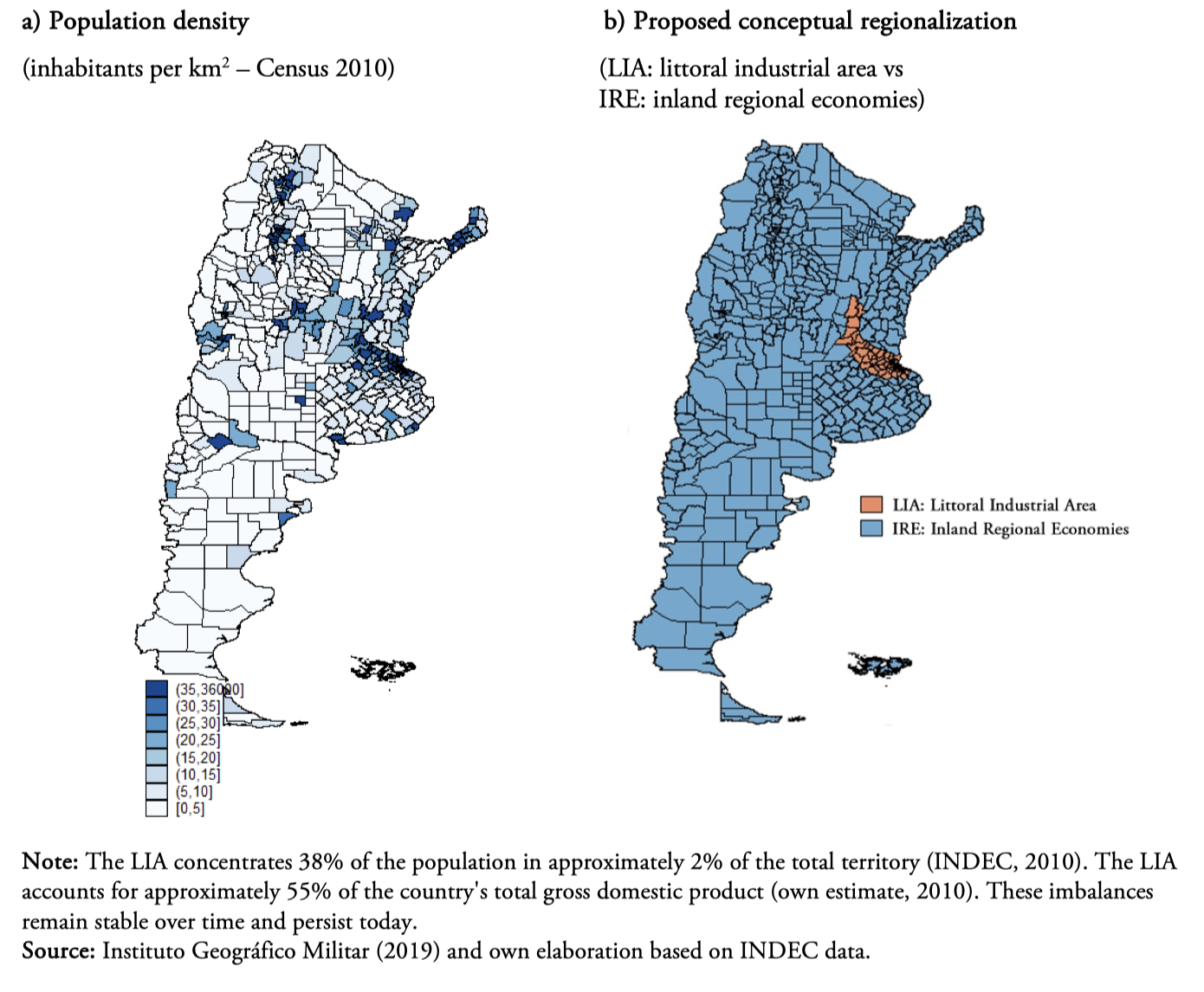
After the First World War and the Great Depression, the world experienced a generalized closure of economies. In Argentina, internal relative prices, managed by the commercial and exchange policy of the national government, punished the inland regional economies (IREs) (Economías Regionales del Interior), favouring the manufacturing concentration in the so-called littoral industrial area (LIA) (Frente Industrial del Litoral).[11] An industrialized seaside area (comparatively rich) and an underdeveloped periphery in the interior (comparatively poor) were consolidating (Figure 2 in Appendix V).
This duality was definitively consolidated during the implementation of the import substitution strategy between 1940 and 1990. Growth (and development) was further concentrated in the LIA, setting up a relationship of dependence of the IREs (Figueras, 1991; Figueras & Arrufat, 2009).
The internationalization of markets has affected the LIA and the IREs in recent decades. The boom in agricultural commodities, given their high relative price, has also had an impact on the IRE in the last two decades (and obviously as a counterpart to the LIA). This has changed the optimal locations per se, leading to new areas of attraction and the abandonment of other areas. We will study this dual situation in our paper, with these contemporary framework conditions.
The measurement of linkages between agglomeration and growth
The empirical literature has identified the variables that are related to economic growth (see Barro, 1991) and has used a regression analysis to estimate its relative influence:
(1)
where g is the vector of economic growth rates and
are explanatory variables.
There are many variables related to economic growth that must be taken into account to avoid omitted variable bias in the estimates of the coefficients. Sala-i-Martin et al. (2004, p. 815) pointed out that “The problem faced by empirical growth economists is that growth theories are not explicit enough about what variables xj belong in the 'true' regression. That is, even if we know what the 'true' model looks like, we do not know exactly what variables xj we should use.”
4.1. The steady-state determinants
We use an empirical framework (based on Barro & Sala-i-Martin, 2004) that relates real per capita product growth to two types of variables: initial levels of state variables, such as the stock of physical capital and the stock of human capital in the forms of educational attainment and health; and control or environmental variables. The study incorporates a set of variables to capture the differences between provinces. Before turning to the econometrics, we focus conceptually on the conditioning variables. Due to information limitations, one cannot consider a variable that, following Thirlwall's law or rule, is crucial to explain the performance of the provinces, specifically their external sales, including their international exports and sales to other provinces.
The economic performance of Argentinian provinces is affected by the transportation cost and the existence of a large consumption centre in the littoral, where the most important port and boarding area is also located. It can be interpreted as the centre in a centre–periphery framework. This economic cost, or virtual distance, has changed over time (and relative distances have certainly changed), but the lack of such crucial data for all jurisdictions over the period of the study unfortunately prevents us from incorporating it. Given that external terms of trade have surely played a role in the last sub-period, its effects are incorporated through a structural change index, a variable constructed considering the different sectoral structures of the provinces. In the study, annual data for the period 1981–2007 for the 23 provinces and the Autonomous City of Buenos Aires[12] are used, for which growth rates for each of the provinces are computed over 10 years.
Regarding the determinants of the steady state included in vector X, the following variables are considered[13]:
Own resources ratio: the share of the total public expenditure financed by the province's own tax resources;
Personnel expenditure ratio: the share of the total public expenditure assigned to personnel spending;
Investment: construction (Gran División 5, in thousands of pesos of 1993) per capita;
Infant mortality rate: the infant mortality rate;
Secondary schooling: the ratio of students enrolled in secondary schools to the population (3 years old and above) attending an educational institution;
Structural change variable: the structural change index.
Two dimensions of human capital are observed: education and health. The ratio of enrolment in secondary schools is an approximation of the educational level, and the infant mortality rate is an approximation of the health status of the population. The participation of construction in the GDP (Gran División 5) is an investment proxy (Investment); although it is a non-reproductive application, this is justified given that construction is the most important item of fixed gross domestic investment. Including the proportion of own tax resources in the total public expenditure of the province (own resources ratio) allows for the identification of provinces that are less dependent on the national government and therefore have a greater capacity to carry out active discretionary policies. In those provinces where the proportion of genuine resources in the total expenditures is higher, greater management capacity and efficiency are expected. The proportion of personnel spending in the province's total expenditure (personnel expenditure ratio) is an indicator of the importance of public employment in the labour market. The structural change variable is defined as follows:
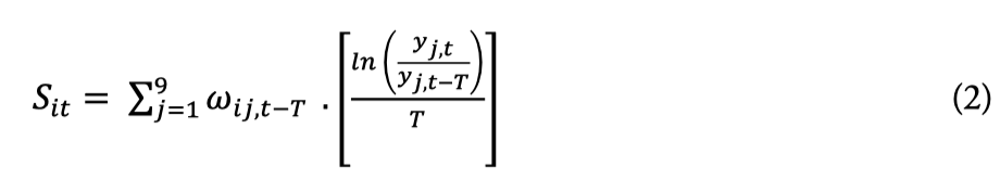
where
is the weight of sector j in province i at time t-T. Note that the structural change variable depends on the growth rates of the sectors and on the lagged values of the sectoral shares, allowing for its treatment as exogenous at the current growth rate of the province's GDP.
This variable measures the effect of exogenous shocks on the growth of each region and is included because these shocks tend to benefit or harm provinces with high or low incomes (which would cause the shocks to be correlated with the explanatory variables) depending on their structure of production. The omission of this variable would tend to bias the estimation of the parameters and the speed of convergence (see Barro & Sala-i-Martin, 2004, pp. 464–472). This variable reveals the rate at which a province would grow if each of the sectors grew at the national average growth rate. When a low value of the variable in a region is observed, it indicates that the province is not growing rapidly due to a negative shock to a sector that is relevant to its economy. One of the shocks that the variable is expected to capture is the regional influence of variations in the terms of trade.
4.2. Agglomeration and growth
The Theil geographic concentration index (agglomeration measure) is used to measure agglomeration. It is calculated, as in Brülhart and Sbergami (2009), from estimates of regional employment as follows:
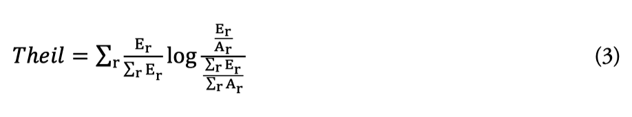
where r denotes a sub-provincial region,
the employment in the region, and Ar the area.
This index is scaled by the regional area, thereby measuring the "topographic concentration": a uniform distribution of employment in the physical space represents "zero agglomeration" and therefore implies a zero Theil geographic concentration index. The larger the deviation of this distribution from uniformity, the higher the value of the index.
In turn, an interaction term with the lagged per capita provincial GDP is used to test the Williamson hypothesis (the effects of increased agglomeration at different levels of economic development). Quadratic terms of the mentioned measures of agglomeration are included to capture possible nonlinear effects.
Estimation
The estimation of the determinants of economic growth (Equation 1) is performed through two alternative methods – a) fixed-effect panel data estimation and b) dynamic GMM estimation – to deal with the possible existence of endogeneity.[14] There is consensus in the literature regarding the superiority of the GMM methodology to fixed-effect models in treating classical econometric problems that arise when dealing with dynamic panel data, particularly socio-economic variables. It can help to reduce endogeneity concerns, simultaneity, and unobserved heterogeneity.[15],[16]
Indeed, Combes and Gobillon (2015) pointed out that one of the strategies that have been used to cope with endogeneity issues in panel data is the GMM approach to estimate the specification in first difference while using lagged values of variables as instruments both in level and in first difference. The approach is valid when the two conditions of relevance and exogeneity of the instruments are verified. Typically, the relevance of instruments is usually not an issue as there is some inertia in local variables and the time span is usually short (a couple of decades at most).
GMM estimation is naturally well suited to dealing with potential endogeneity issues; therefore, it aims to isolate the effect from agglomeration to growth.[17] Indeed, dynamic GMM remains consistent even if some variables, such as agglomeration, are endogenous if the instrumental variables are lagged. Another advantage of dynamic GMM estimation is that time-invariant measurement error is absorbed into region-specific effects and allows dynamic panel GMM to remain consistent even in the presence of a province–year-specific measurement error provided that it is serially uncorrelated. Appendix II presents a brief discussion of this estimation technique.
5.1. Fixed effects and GMM results
Table 1 presents panel data estimations of the determinants of growth. The 10-year growth rate of the real GDP is related to two types of variables: first, initial levels of state variables, such as human capital in the forms of educational attainment and health (secondary schooling and the infant mortality rate); and, second, control variables, such as investment, the personnel expenditure ratio, the own resources ratio, and a structural change variable, including the variables that are linked to agglomeration: agglomeration measure, agglomeration*GDP, and agglomeration squared. Even columns show the results for the full model, including all the regressors, and odd columns report comparable estimates without investment.
In Table 1 (Columns 2–4), the fixed-effect estimates are presented (Hausman test χ2(17)=90.79, p-value=0.000; χ2 (17)=86.77, p-value=0.000, respectively). There is also evidence of cross-sectional dependence (Pesaran test 8.263, p-value=0.000; 8.989, p-value=0.000) and of groupwise heteroscedasticity (Wald test χ2 (24)=11591.6, p-value=0.000; test χ2=94926.95, p-value=0.000, respectively), so Columns 3–4 present estimations using Driscoll and Kraay standard errors (Hoechle, 2007). Random-effect estimates are not presented as the Hausman test indicates that those results are inconsistent.
Given that it has been pointed out that growth and geographic concentration can be treated as a self-reinforcing process (Fujita & Thisse, 2002, p. 391; Martin & Ottaviano, 1999, p. 948), we focus on GMM estimation to deal with the causal effect that runs from agglomeration to growth. The test for first-order serial correlation rejects the null of no first-order serial correlation, but it does not reject the null that there is no second-order serial correlation. It is standard to run tests of overidentifying restrictions after dynamic panel GMM estimation. We report the Hansen test statistic and its associated p-value, which is satisfactory in both estimations. Furthermore, we limit the maximum lag length of the instrument set to one.
The results vary significantly depending on the estimation method. Table 1 reports the results using two approaches to specifications (fixed effects (FE) without and with Driscoll–Kraay standard errors and two-step GMM estimation). Moving from FE to GMM has a significant impact on the statistical significance (but not on the sign) of the measured speed of convergence. In the specifications with FE (Estimations 1–4), the coefficient of the agglomeration measure is negatively signed and significant, and the interactions with the per capita GDP (agglomeration*GDP) and agglomeration squared are both positive and significant, suggesting a reverse Williamson hypothesis. Conversely, the two-step GMM estimates[18] yield a coefficient of the agglomeration measure that is positively signed, and its significance depends on whether the specification includes the investment variable. As investment is not significant, specification (5) is preferred to specification (6). The interaction with the per capita GDP (agglomeration*GDP) results as significant and negatively signed, whereas agglomeration squared is positive although not significant. This result supports the existence of a systematic relationship between agglomeration and growth, as in the Williamson hypothesis, and is in line with the results of other studies (Aroca et al., 2018; Barrios & Strobl, 2009; Guevara 2016; Lessmann, 2014).
The ratio of enrolment in secondary schools measures schooling. Since this variable is predetermined, it enters as its own instrument in the GMM regressions. The estimated coefficient is positive and significant throughout the estimations but increases in importance in the GMM estimations. The estimated coefficient is highly significant (0.00483 in Estimation 6), and it means that an increase in schooling raises the GDP growth rate of the provinces. The other human capital variable considered in the empirical estimation is the infant mortality rate, which is also predetermined; hence, it enters as its own instrument in the GMM regressions as an approximation of the evolution of the health status of the population. This indicator is not significant in all the specifications.
The effect of the proportion of own tax resources to the total public expenditure of the province (own resources ratio) on growth retains its positive sign across specifications but is only significant in the case of fixed effects with Driscoll–Kraay S.E. (Estimations 3 and 4), showing that, in those provinces where the proportion of own genuine resources in the total expenditures is higher, there is greater management capacity and efficiency.
The proportion of personnel spending in a province's total expenditure (personnel expenditure ratio) is an indicator of the importance of public employment in the labour market. The associated coefficient is not significant across specifications. The participation of construction in the GDP (Gran División 5) is used as an investment proxy (investment), a variable that is treated as predetermined in the GMM. The estimated coefficient is highly unstable, being positive and statistically significant in the fixed-effect specifications and negative and non-significant in the case of the GMM estimates.
The structural change variable shows a significant and positive influence, which implies that exogenous shocks affect the growth rate of the provinces substantially. These exogenous shocks have different effects in different provinces, depending on the economic structure of their GDP. For example, Figueras et al. (2014) observed at least two periods in which the different effects become more acute: one of these periods is the time of the economic opening of the 1990s, and the other is the period of the commodity price boom in the first decade of this century.
Table 1.
Estimates of the determinants of growth – Panel data
| Dependent variable: 10-year GDP growth rate | Fixed effects (1) | Fixed effects (2) | Driscoll– Kraay (3) | Driscoll– Kraay (4) | Two–step GMM (5) | Two–step GMM (6) |
| Lagged GDP | 0.660*** | 0.621*** | ||||
| (0.162) | (0.155) | |||||
| Initial GDP | -0.0824*** | -0.0840*** | -0.0824*** | -0.0840*** | -0.00539 | -0.00831 |
| (0.00450) | (0.00457) | (0.00436) | (0.00433) | (0.00450) | (0.00848) | |
| Personnel expenditure ratio | 0.0109 | 0.00797 | 0.0109 | 0.00797 | -0.0201 | 0.00834 |
| (0.0109) | (0.0110) | (0.00636) | (0.00541) | (0.0460) | (0.0649) | |
| Own resources ratio | 0.0251 | 0.0267 | 0.0251*** | 0.0267*** | 0.0465 | 0.0647 |
| (0.0166) | (0.0166) | (0.00851) | (0.00936) | (0.0304) | (0.0633) | |
| Secondary schooling | 0.00139** | 0.00137** | 0.00139* | 0.00137* | 0.00451** | 0.00483*** |
| (0.00055) | (0.00055) | (0.00074) | (0.00071) | (0.00180) | (0.00172) | |
| Infant mortality rate | 1.82e-05 | 1.02e-05 | 1.82e-05 | 1.02e-05 | 0.000276 | 0.000320 |
| (7.42e-05) | (7.41e-05) | (3.91e-05) | (3.97e-05) | (0.000204) | (0.00023) | |
| Structural change variable | 0.186*** | 0.178*** | 0.186** | 0.178** | 0.337** | 0.320* |
| (0.0360) | (0.0362) | (0.0742) | (0.0747) | (0.159) | (0.170) | |
| Agglomeration measure | -0.284*** | -0.252*** | -0.284*** | -0.252*** | 0.0948* | 0.0592 |
| (0.0577) | (0.0599) | (0.0795) | (0.0781) | (0.0532) | (0.0649) | |
| Agglomeration*GDP | 0.0309*** | 0.0294*** | 0.0309** | 0.0294** | -0.0238*** | -0.0194** |
| (0.00494) | (0.00499) | (0.0132) | (0.0131) | (0.00794) | (0.00871) | |
| Agglomeration squared | 0.0876** | 0.0717** | 0.0876*** | 0.0717*** | 0.00451 | 0.0128 |
| (0.0354) | (0.0362) | (0.0266) | (0.0242) | (0.0283) | (0.0283) | |
| Investment | 1.43e-06* | 1.43e-06*** | -2.64e-06 | |||
| (7.61e-07) | (4.16e-07) | (4.41e-06) | ||||
| Constant | 0.393*** | 0.395*** | 0.393*** | 0.395*** | ||
| (0.0240) | (0.0240) | (0.0196) | (0.0196) | |||
| Time dummies | yes | yes | yes | yes | yes | yes |
| Observations | 406 | 406 | 406 | 406 | 406 | 406 |
| ar1 | -2.870 | -3.185 | ||||
| ar1p | 0.00411 | 0.00145 | ||||
| ar2 | 0.556 | 0.600 | ||||
| ar2p | 0.578 | 0.549 | ||||
| Hansen | 3.739 | 3.691 | ||||
| Hansenp | 0.809 | 0.815 | ||||
| F | 127.4 | 121.4 | 23196 | 25248 |
Agglomeration and growth in Argentinian provinces
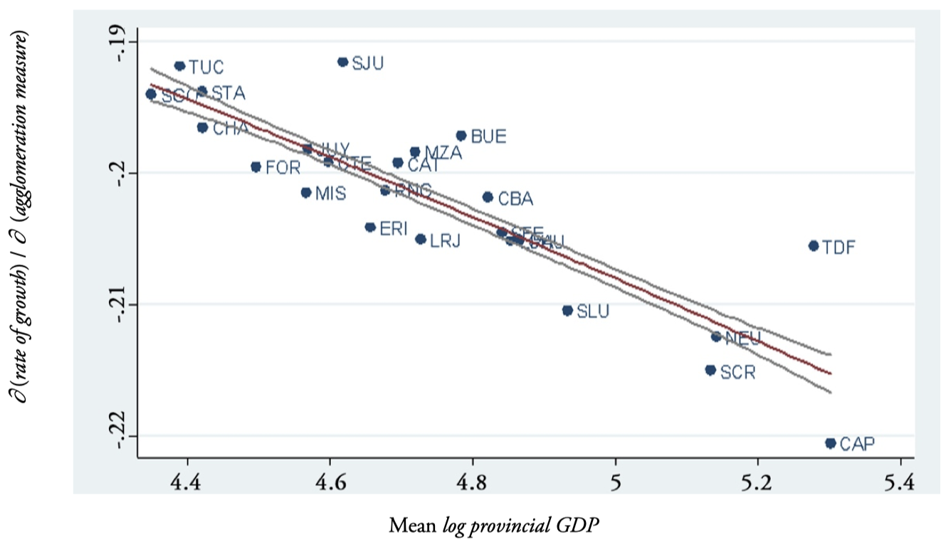
The Williamson hypothesis implies an inverted-U relationship between growth and agglomeration. The derivative of the rate of growth with respect to the agglomeration measure, for each income level – in the complete range of this inverted-U relationship – would intercept zero, with a "positive" section and a "negative" one. Agglomeration mainly exerts a positive influence at the early stages of development, when the transportation and communication infrastructures are weak and the access to capital markets is limited, so efficiency can be increased significantly by the spatial concentration of production. Later, when the infrastructure quality improves and markets expand, the negative externalities of congestion can promote a more geographically dispersed economy.
Figure 1 illustrates this relationship between the per capita GDP and the derivative of growth with respect to the agglomeration measure, that is, how growth changes when agglomeration changes. The derivative of growth with respect to the Theil geographic concentration index is calculated based on the results in Table 1 (Specification (5) – two-step GMM). In particular, it can be observed that Argentinian provinces are in the descending section of the Williamson curve (Figure 1).[19] The data suggest that agglomeration diseconomies are in place during the period under study: the higher the level of income, the more negative the agglomeration influence on the GDP growth rate. This implies that, according to the measure of agglomeration that is used, Argentinian provinces are (during this period) at a stage of development at which agglomeration conspires against growth, hence contributing to convergence. At this stage, when the productive advantage of large cities is constantly eroded, it could be sustained by new job creation and innovation (Duranton, 2014).
The results show that the level of development (or income) is a relevant variable when analysing the relationship between growth and agglomeration, as Williamson (1965) indicated. We could hypothesize here that Henderson’s (2003) assertion about the influence of national policies and institutions on urban concentration is verified in the case of the Argentinian provinces. Henderson found that Argentina, Mexico, and Thailand are among the most concentrated countries, having traditionally centralized governments, where the effect of trade policies and certain intra-regional factors (such as institutions) may have considerable importance.
Previously, Ades and Glaeser (1995) considered the same factors but found strong results of the presence of political power over urbanization given that the proximity to the centre of political decision making increases the political influence. The pressure of the capital area’s population induces the government to extract wealth from the interior areas and apply those resources in favour of the capital area, and these income transfers attract immigrants, promoting concentration (then there is a circular and, perhaps, perverse relationship from the economic and political points of view).
Conclusions
This work analyses the link between the phenomenon of growth and the spatial concentration in the regional context with data from the Argentinian provinces for the period 1981–2007. To test the Williamson hypothesis, the estimation of the determinants of economic growth is performed through two alternative methods: fixed effects and dynamic GMM. The choice of the estimation approach is crucial. When controlling for potential simultaneity bias, the relationship between agglomeration and growth is observed in the case of Argentinian provinces. This suggests that the original Williamson hypothesis is in place, meaning that agglomeration boosts GDP growth up to a certain level of economic development. When this endogeneity is not accounted for (fixed-effect estimates), it seems that a reverse Williamson hypothesis applies.
In particular, for the period studied, it is observed that Argentinian provinces are in the descending section of the Williamson curve (Figure 1).[20] The data analysis suggests two things: (a) that agglomeration diseconomies are in place; the higher the levels of income, the more negative the association between agglomeration and the GDP growth rate; and (b) that the Argentinian provinces are (in the period of the study) at a stage of development in which agglomeration conspires against growth, hence contributing to convergence (areas with more concentration and development would grow less).
It is at this stage, when the productive advantage of large cities is constantly eroding, that growth could be sustained by creating new jobs and innovation (Duranton, 2014). As Martin and Ottaviano (2001) highlighted, the same factors that spur growth also trigger agglomeration, and the cumulative process reinforces the effect that a change in one of these factors has on growth and agglomeration. Furthermore, it was found that, when endogeneity is controlled, the GDP convergence between the Argentinian provinces is less evident and the influences of human capital and structural change on growth estimated through the GMM become stronger.
Finally, a question that opens up a future research agenda is whether the agglomeration is an inevitable process per se or whether it is feasible to "manipulate" the level of agglomeration (through economic policies) according to the growth target. Policymakers face the challenge of turning urban systems into drivers of economic growth, especially in the case of developing countries (such as Argentina).
Certainly, another relevant point to investigate is the issue raised by Ades and Glaeser (1995), who suggested that urban concentration may result from attempts to maximize political power (especially by some political groups) and, therefore, generate a process of distortion (leading to a greater concentration level than the optimal one).
Annexes
Appendix I
Dependent variable: 10-year GDP growth.
GDP: Per capita real provincial gross domestic product. Base=1993. Source: own elaboration based on data from Consejo Federal de Inversiones (CFI) and Russo (1997). Period 1981–2010 (annual). CFI data retrieved from http://www.biblioteca.cfi.org.ar.
Agglomeration variables
Agglomeration measure: Theil geographic concentration index for the intra-province spatial distribution of employment, following Brülhart and Sbergami (2009) and assuming a production function characterized by uniform labour productivity within each province. Source: authors’ calculations based on INDEC data. Period 1991–2007 (annual). INDEC data retrieved from https://www.indec.gob.ar.
Control variables
Initial GDP: The initial level of provincial per capita GDP (log in base 10). Period 1981–2007 (annual).
Secondary schooling: The provincial ratio of enrolment in secondary schools to the total population. Source: Census of Population and Housing, INDEC. Period: 1980, 1991, and 2001 (annual). Retrieved from https://www.indec.gob.ar.
Infant mortality rate: The provincial ratio of the number of deaths of children under 1 year of age per 1000 live births. Source: Direction of Statistics and Health Information, Ministry of Health. Period 1981–2007 (annual). Retrieved from https://www.argentina.gob.ar/salud/deis.
Own resources ratio: Own fiscal resources as a share of the total provincial government expenditure. Source: CFI. Period 1981–2007 (annual).
Personnel expenditure ratio: Personnel government expenditure as a share of the total provincial government expenditure. Source: CFI. Period 1981–2007 (annual).
Structural change variable: Structural change index. Source: authors’ calculations based on INDEC and CFI data. Period 1981–2007 (annual).
Investment: Construction. Source: own elaboration based on data from Consejo Federal de Inversiones (CFI) and Russo (1997). Gran División 5 (ClaNAE 1997). The results are assimilable to the F-Construction section of the International Standard Industrial Classification Third Revision (ISIC Rev. 3).
Appendix II
The growth regression can be written as:
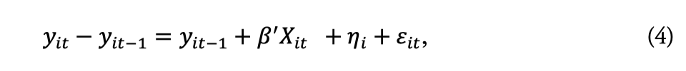
where is the 10-year growth of the real per capita GDP, X represents the set of explanatory variables, other than the lagged per capita GDP, is an unobserved province-specific effect, is the error term, and the subscripts i and t represent the province and time, respectively.
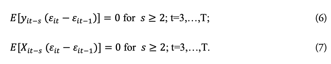
Arellano and Bond (1991) proposed to take the equation in differences, thus eliminating the province-specific effect:

This change introduces a new bias: given its construction, the new error term is correlated with the lagged dependent variable . The estimation method relies on the assumptions that (a) the error term is not serially correlated and (b) the explanatory variables are uncorrelated with future realizations of the error term. The moment conditions are:
Arellano and Bond (1991) proposed a two-step GMM estimator. In the first step, the error terms are assumed to be independent and homoscedastic across is (in our case, the provinces) and over time. In the second step, the residuals obtained in the first step are used to construct a consistent estimate of the variance–covariance matrix, thus relaxing the assumptions of independence and homoscedasticity. The two-step estimator is thus asymptotically more efficient than the first-step estimator.
Arellano and Bond’s (1991) regression equations are therefore expressed in terms of first differences, and endogenous explanatory variables are instrumented with suitable lags of their own levels. If the lagged levels are weakly correlated with the differences in the explanatory variables, then they are weak instruments for the first-differences variables and the first-step estimator, so finite sample bias may still occur.
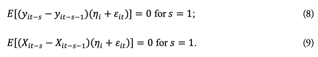
To reduce the potential bias from the difference estimator, Arellano and Bover (1995) and Blundell and Bond (1998) used an estimator that combines the regression in differences with the regression in levels in a system. In this panel data GMM estimator, the regression equations are in levels and the additional instruments are expressed in lagged differences. These are appropriate instruments under the following additional assumption: although there may be a correlation between the levels of the right-hand side variables and the province-specific effect, there is no correlation between the differences of these variables and the province-specific effect.[21]
Given that lagged levels are used as instruments in the regression in differences, only the most recent difference is used as an instrument in the regression in levels. Using additional lagged differences would result in redundant moment conditions (Arellano & Bover, 1995). Thus, additional moment conditions for the second part of the system (the regression in levels) are:
The use of a GMM estimation strategy aims to isolate the potential influence of agglomeration on growth. While it is a valid tool to reduce endogeneity, it is necessary to recognize that it is a sub-optimal tool. Indeed, dynamic GMM panel estimation remains consistent even if some of the variables, as agglomeration, are endogenous if the instrumental variables are lagged. Another advantage of dynamic GMM estimation is that the time-invariant measurement error is absorbed into region-specific effects, allowing the dynamic panel GMM to remain consistent even in the presence of province–year-specific measurement error provided that it is serially uncorrelated.
The consistency of the GMM estimators depends on whether the lagged values of the explanatory variables are valid instruments in the growth regression. Two specification tests are considered. The first one examines the null hypothesis that the error term is not serially correlated. The model specification is supported when the null hypothesis is not rejected. In the system specification, we test whether the differenced error term is second-order serially correlated. First-order serial correlation of the differenced error term is expected even if the original error term (in levels) is uncorrelated unless the latter follows a random walk. Second-order serial correlation of the differenced residual indicates that the original error term is serially correlated and follows a moving average process of at least order one. This would reject the appropriateness of the proposed instruments. The second test is a Hansen test of overidentifying restrictions under conditional heteroscedasticity, which tests the overall validity of the instruments by analysing the sample analogue of the moment conditions used in the estimation process. Failure to reject the null hypothesis gives support to the model.
Appendix III
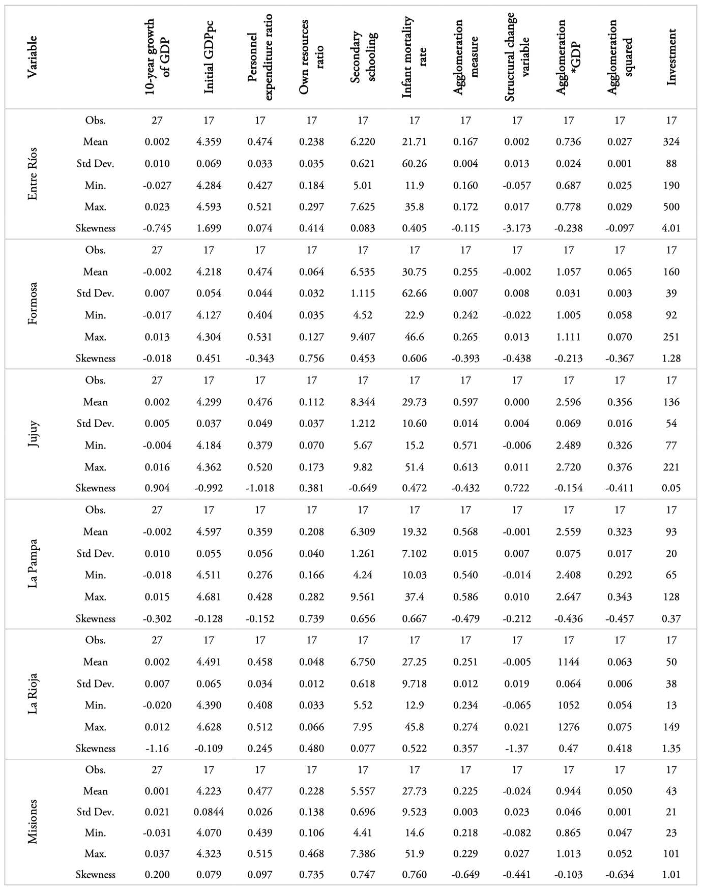
3.a. Descriptive statistics
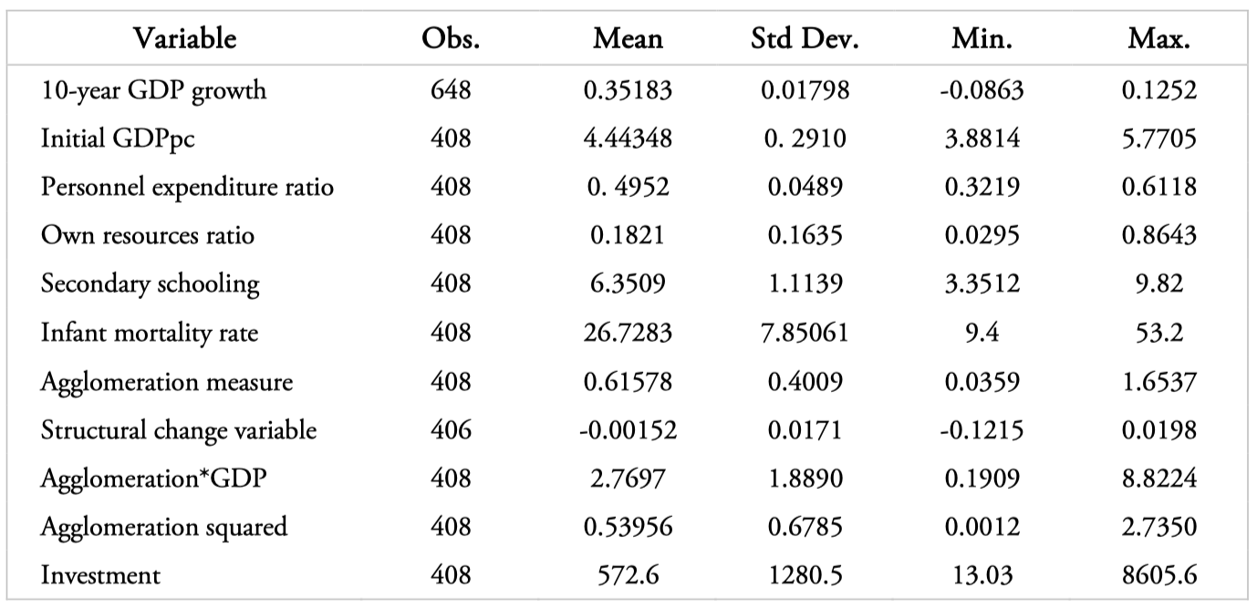
Note: See Appendix I for a description of the variables, units of measurement, and sources.
3.b. Correlation matrix
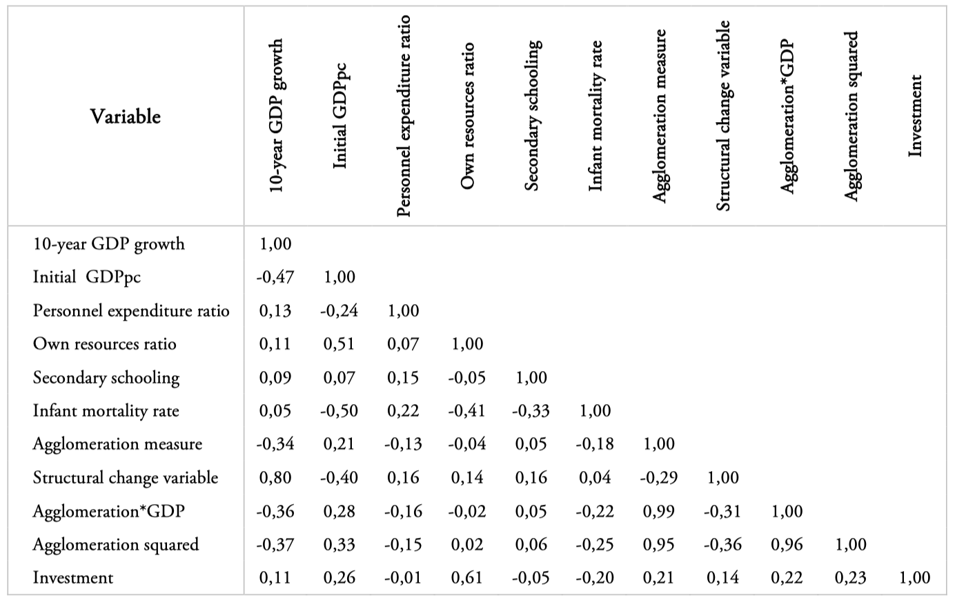
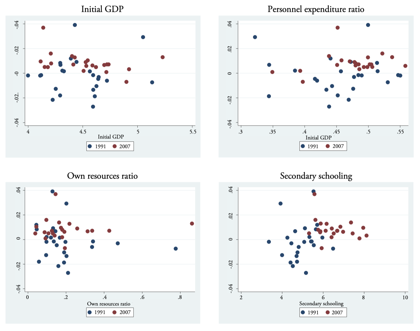
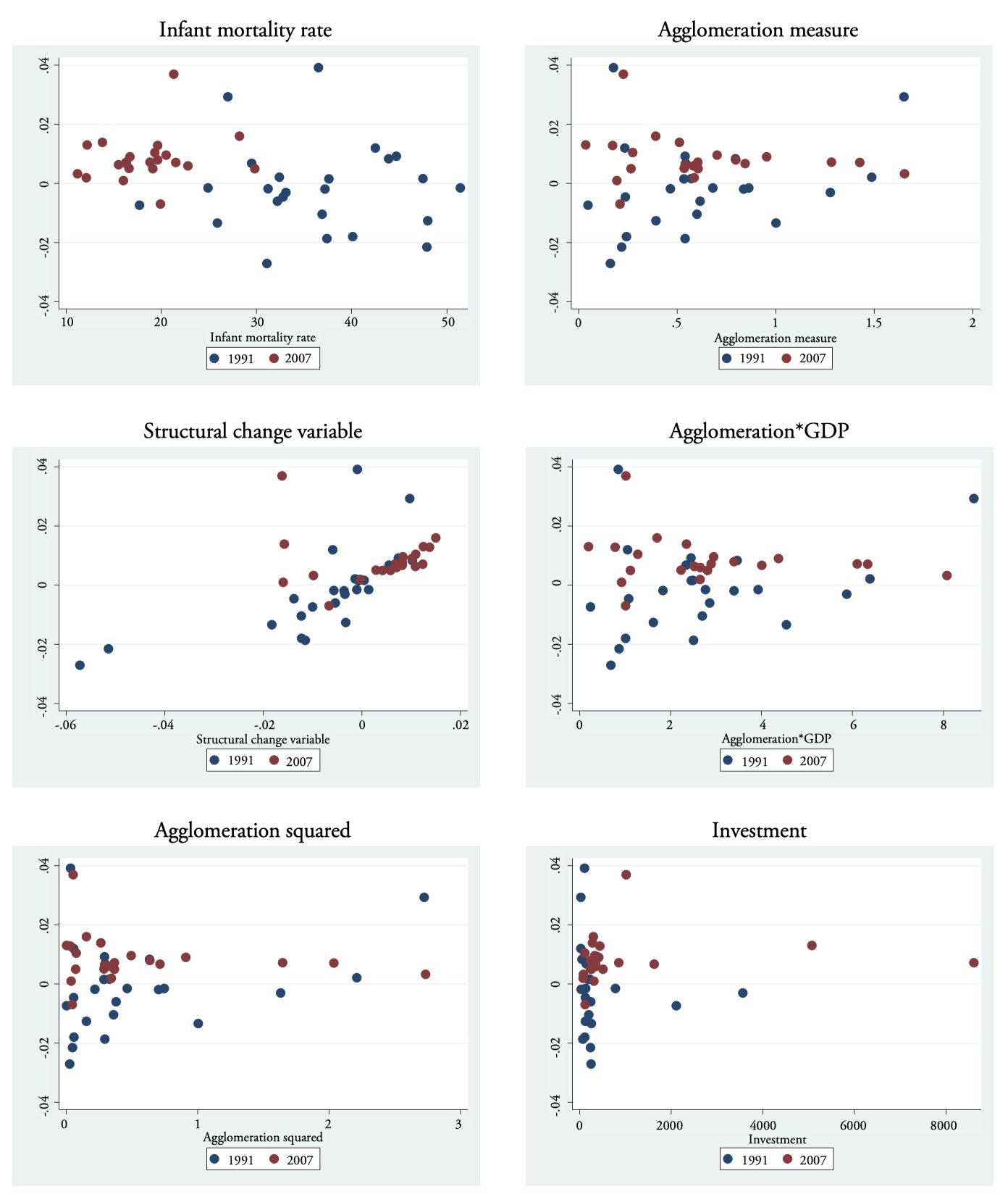
3.c. Scatter plots – Dependent variable 10-year growth of GDP and variables of interest
Appendix IV
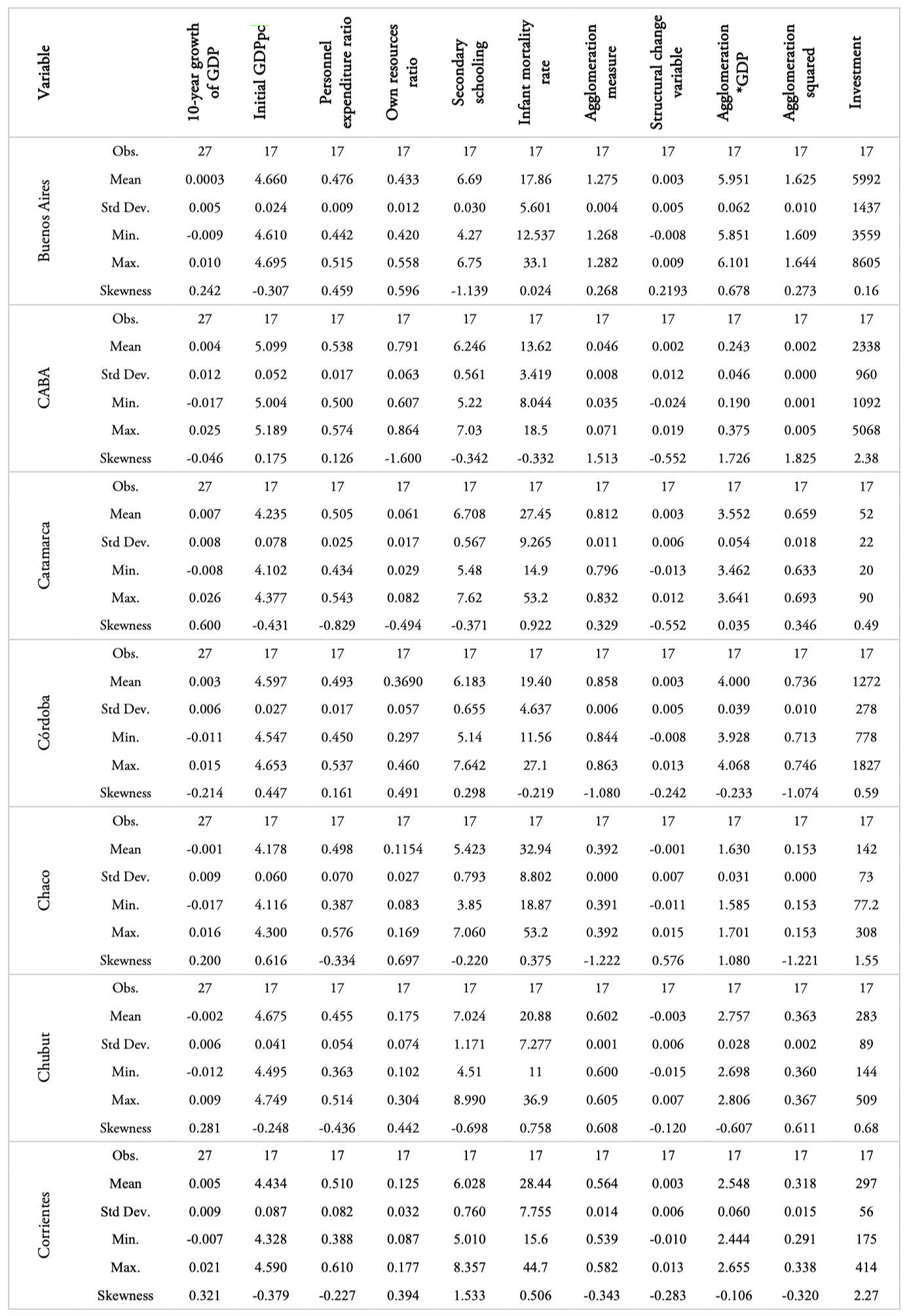
4.a. Descriptive statistics by province (first part)
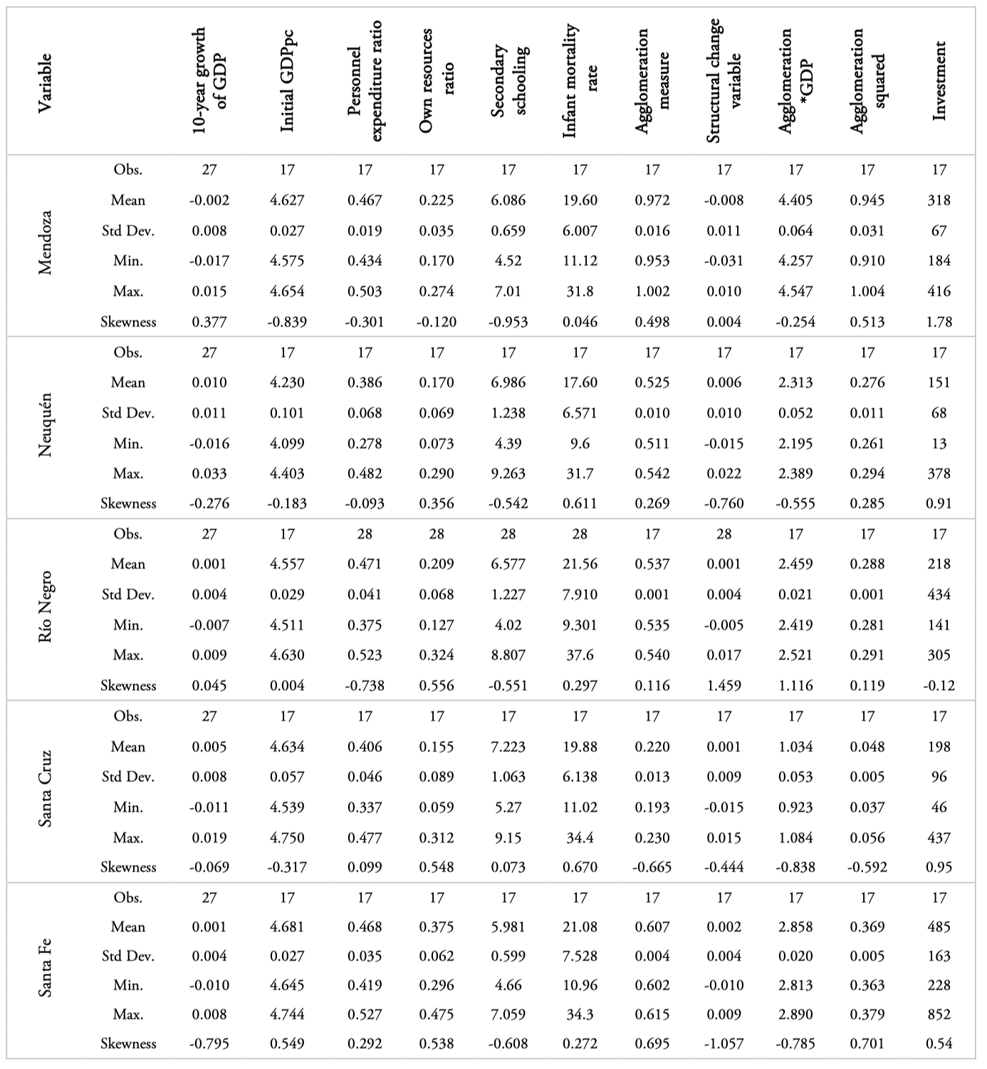
4.a. Descriptive statistics (second part)
4.a. Descriptive statistics (third part)
4.a. Descriptive statistics (fourth part)
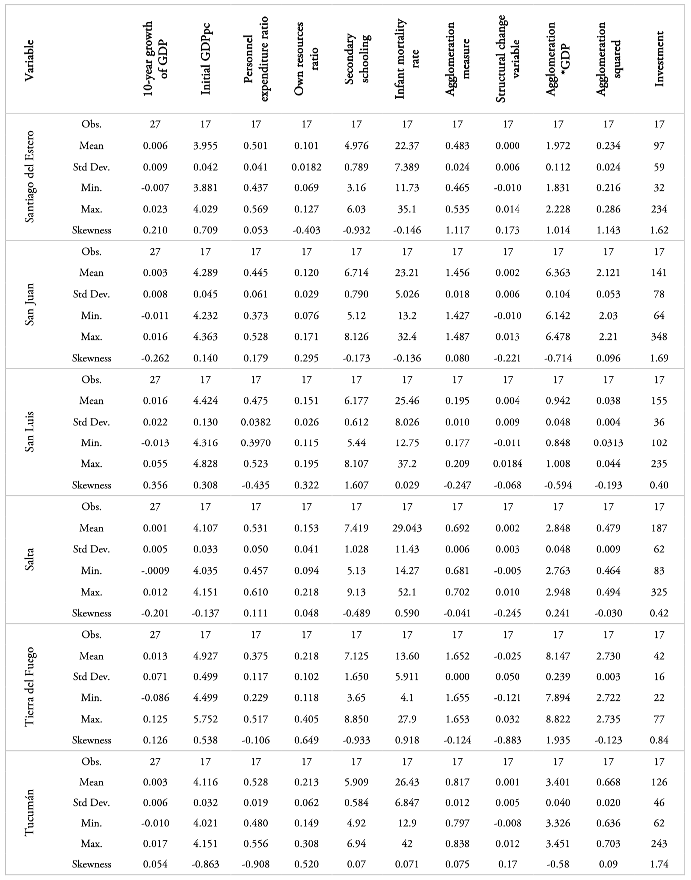
Note: See Appendix I for a description of the variables, units of measurement, and sources.
Appendix V
Figure 2.
Descriptive maps – Evolution of the territorial organization
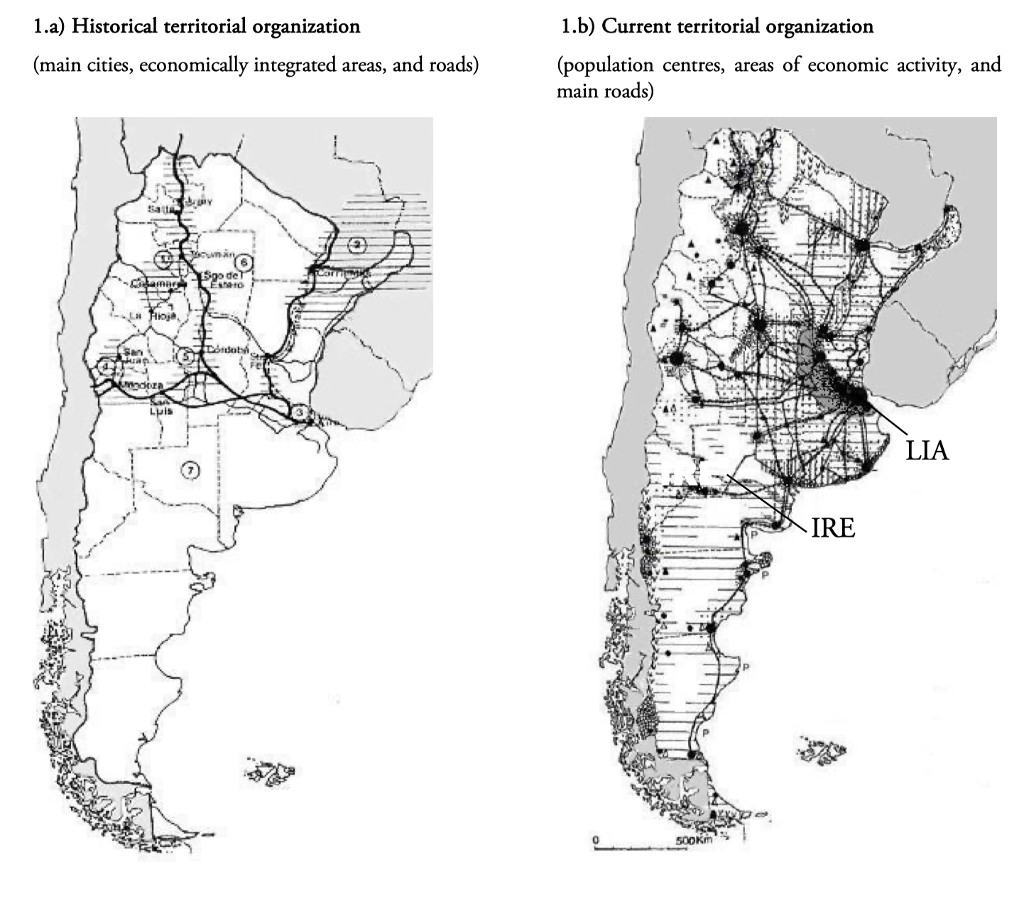
Note: The legends IRE and LIA are additional modifications to the original image. LIA: littoral industrial area. IRE: inland regional economies. Source: Roccatagliata (1988, pp. 118 and 126).
Figure 3.
Descriptive maps – Main variables at the provincial level (second part)
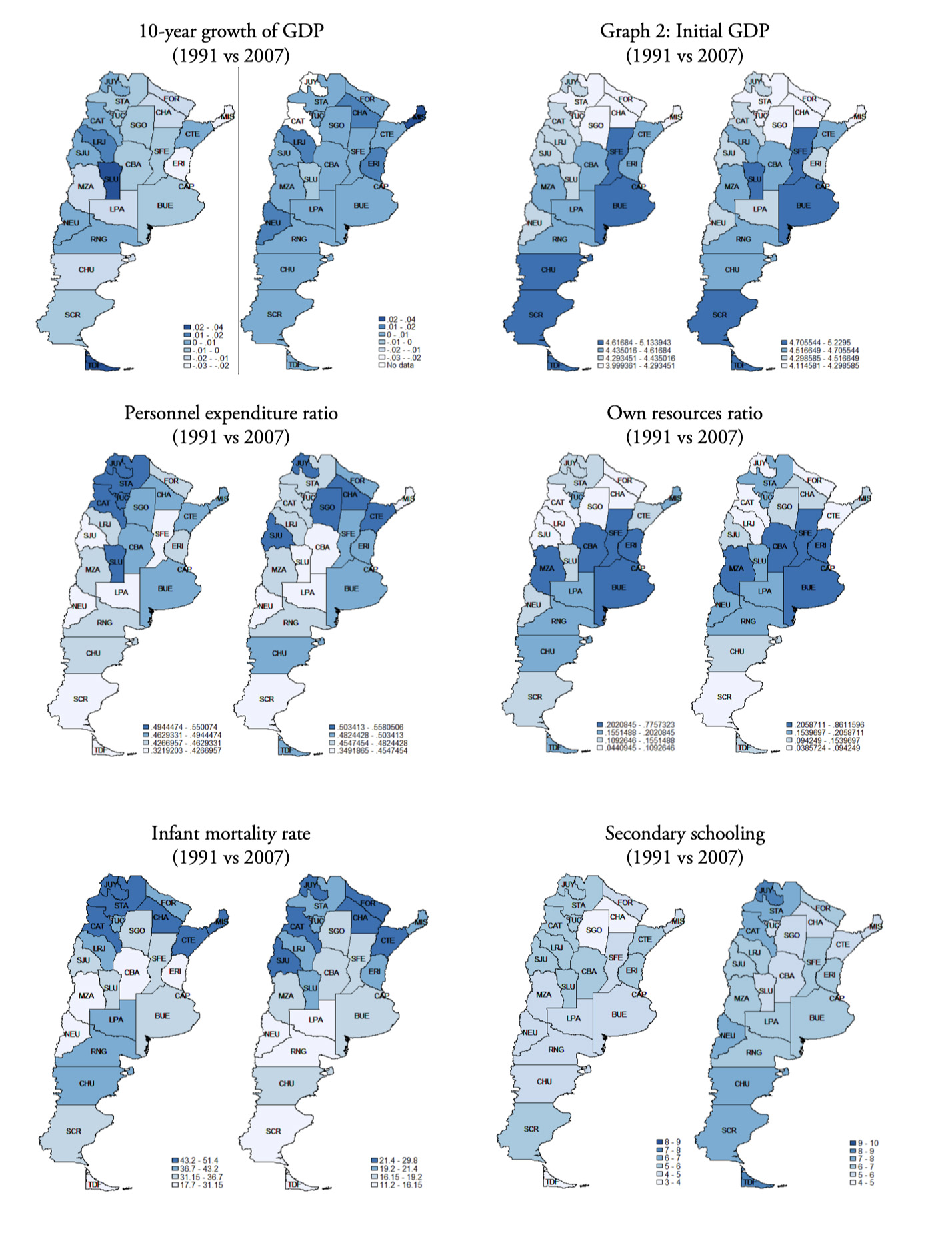
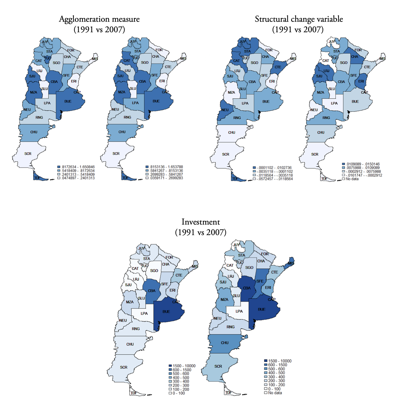
Note: See Appendix I for a description of the variables, units of measurement, and sources. Source: Instituto Geográfico Militar (2019) and own elaboration based on INDEC and CFI data. Importar tabla Codes used in the maps
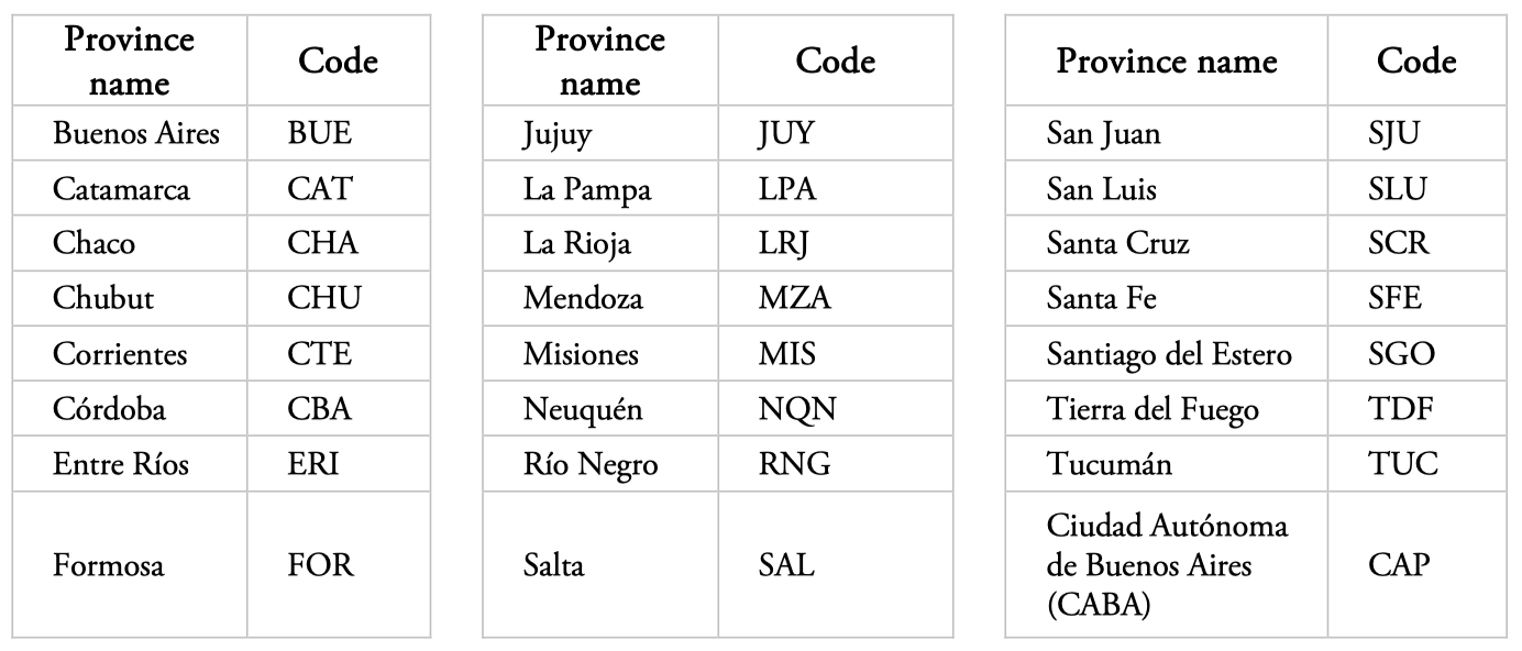
Note: Malvinas, South Georgia Islands, and South Sandwich Islands, currently occupied by the United Kingdom, although not charted, are part of the Province of Tierra del Fuego, Argentina.
Figure 4.
Description of territorial organization by provincial regional subdivision (departments)
References
Ades, A.F., & Glaeser, E. (1995). Trade and Circuses: Explaining Urban Giants. Quarterly Journal of Economics 110(1), 195-227.
Amos, O. (1988). Unbalanced regional growth and regional income inequality in the latter stages of development. Regional Science and Urban Economics, 8(4), 549-566.
Arellano, M., & Bond, S. (1991). Some tests of specification for panel data: Monte Carlo evidence and an application to employment equations. The Review of Economic Studies, 58, 277 – 297.
Arellano, M., & Bover, O. (1995). Another look at the instrumental variable estimation of error-components models. Journal of Econometrics, 68(1), 29-51.
Aroca, P., Azzoni, C., & Sarrias, M. (2018). Regional concentration and national economic growth in Brazil and Chile. Letters in Spatial and Resource Sciences, 11(3), 343–359.
Atkinson, A. (1997). Bringing income distribution in from the cold. Economic Journal, 107(441), 297-321.
Baltagi, B. (2013). Econometric Analysis of Panel Data, 5th Edition Wiley.
Barrios, S., & Strobl, E. (2009). The dynamics of regional inequalities. Regional Science and Urban Economics, 39(5), 575-591.
Barro, R., & Sala-i-Martin, X. (2004). Economic Growth. MIT Press.
Barro, R.J. (1991). Economic Growth in a Cross Section of Countries. Quarterly Journal of Economics, 106(2), 407-443.
Barro, R.J., & Lee, J. W. (1994). Sources of economic growth. In Carnegie-Rochester conference series on public policy (Vol. 40, June, pp. 1-46). North-Holland.
Becattini, G., Costa, M., & Trullén, J., (2002). Desarrollo local: teorías y estrategias. Ed. Civitas.
Bellandi, M. (1986). El distrito industrial en Alfred Marshall. Estudios Territoriales 20, 31-44.
Bernedo Del Caprio, M., & Patrick, C. (2017). Agglomeration and informality: Evidence from peruvian firms. Andrew young School of policy studies (Research Paper Series. 17‐13).
Blundell, R., & Bond, S. (1998). Initial conditions and moment restrictions in dynamic panel data models. Journal of Econometrics, 87(1), 115-143.
Brülhart, M., & Sbergami, F. (2009). Agglomeration and growth: Cross-country evidence. Journal of Urban Economics 65, 48–63.
Castells-Quintana, D. (2017). Malthus living in a slum: Urban concentration, infrastructure and economic growth. Journal of Urban Economics, 98, 158-173.
Chauvin, J.P., Gleaser, E., Ma, Y., & Tobio, K. (2017). What is different about urbanization in rich and poor countries? Cities in Brazil, China, India, and United States. Journal of Urban Economics, 98, 17–49.
Ciccone, A., & Hall, R. (1996). Productivity and the Density of Economic Activity. The American Economic Review, 86(1), 54-70.
Ciccone, A. (2002). Agglomeration effects in Europe. European Economic Review, 46(2), 213-227.
Combes, P., & Gobillon, L. (2015). The Empirics of Agglomeration Economies. Chapter 5, p. 247-348. Elsevier.
Combes, P.P., Lafourcade, M., Thisse, J., & Toutain, J.C. (2011). The rise and fall of spatial inequalities in France: A long-run perspective. Explorations in Economic History, 48(2), 243-271.
Combes, P. P., & Gobillon, L. (2015). The empirics of agglomeration economies. In J. V. Henderson & J.‐F. Thisse (Eds.), Handbook of regional and urban economics (Vol. 5, pp. 247–348). Elsevier‐North‐Holland.
Datt, G., & Ravallion, M. (2002). Is India's Economic Growth Leaving the Poor Behind? Journal of Economic Perspectives, 16(3), 89-108.
Diez-Minguela, A., Martinez-Galarraga, J., & Tirado-Fabregat, D. (2018). Regional Inequality in Spain. Palgrave Macmillan.
Dixon, R., & Thirwall, A. (1975). A model of regional growth rate differentials along Kaldorian lines. Oxford Economic Papers, 1975, 27(3), 297-308.
Duranton, G. (2008). Viewpoint: From cities to productivity and growth in developing countries. Canadian Journal of Economics, 41(3), 689-736.
Duranton, G. (2014). Growing through cities in developing countries. Policy Research Working Paper Series 6818, The World Bank.
Duranton, G. (2016). Agglomeration effects in Colombia. Journal of Regional Science, 56(2), 210–238.
Duranton, G., & Puga, D. (2004). Micro-foundations of urban agglomeration economies. In Henderson, V., Thisse, J.F. (Editors) Handbook of Regional and Urban Economics (Vol.4). North-Holland.
Figueras, A., Cristina, D., Blanco, V., Iturralde, I., & Capello, M. (2014). Un aporte al debate sobre la convergencia en Argentina; la importancia de los cambios estructurales. Revista Finanzas y Política Económica, Vol. 6(2), 287-316.
Figueras, A. (1991). Reflexiones económicas sobre la economía espacial argentina. Reunión AAEP, Santiago del Estero.
Figueras, A., & Arrufat, A. (2009). El desafío del Territorio, Ed. ACFCE.
Friedmann, J. (1972). A general theory of polarized development. In Growth Centres in Regional Economic Development (pp. 82-107). Ed. N. M. Hansenpp.
Fujita, M., & Thisse, J.-F. (2002): Economics of Agglomeration. Cities, Industrial Location and Economic Growth, Cambridge University Press.
Gardiner, B., Martin, R., & Tyler, P. (2010). Does spatial agglomeration increase national growth? Some evidence from Europe. Journal of Economic Geography, 11(6), 979–1006.
Glaeser, E.L., & Resseger, M.G. (2010). The Complementarity between Cities and Skills. Journal of Regional Science, 50(1), 221–244.
Glaeser, E.L., & Gottlieb, J.D. (2009). The wealth of cities: agglomeration economies and spatial equilibrium in the United States. Journal of Economic Literature 47, 983-1028.
Guevara, C. (2016). Growth Agglomeration Effects in Spatially Interdependent Latin American Regions. GATE Working Paper No. 1611.
Henderson, J.V. (2000). The Effects of Urban Concentration on Economic Growth. NBER Working Paper No. 7503.
Henderson, J.V. (2003). The urbanization process and economic growth: The so-what question. Journal of Economic Growth 8(1), 47–71.
Henderson, J.V. (2010). Cities and Development. Journal of Regional Science, 50(1), 515-540.
Henderson, V. (2002). Urbanization in developing countries. The World Bank Research Observer, 17(1), 89-112.
Hoechle, D. (2007). Robust standard errors for panel regressions with cross-sectional dependence. Stata Journal, 7(3), 281.
IGN, Instituto Geográfico Nacional de la República Argentina (2019). Provincias de la República Argentina: División político territorial de primer orden, incluye la Ciudad Autónoma de Buenos Aires (CABA). Shapefile archive. Creation date 26-04-2019. Catálogo de objetos geográficos IGN, Dirección de Información Geoespacial. Buenos Aires. Retrieved December 1, 2020 from: https://www.ign.gob.ar/NuestrasActividades/InformacionGeoespacial/CapasSIG
Jedwab, R., Christiaensen, L., & Gindelsky, M. (2017). Demography, urbanization and development: Rural push, urban pull and… urban push? Journal of Urban Economics, 98, 6-16.
Kaldor, N. (1955). Alternative Theories of Distribution. The Review of Economic Studies, 23(2), 83–100.
Kaldor, R. (1970). The case for regional policies. Scottish Journal of Political Economy, 17, 337-347.
Krätke, S. (2004). Urbane Ökonomien in Deutschland: Clusterpotenziale und globale Vernetzungen. Zeitschrift für Wirtschaftsgeographie, 48, 146–163.
Kuznets, S. (1955). Economic growth and income inequality. American Economic Review, 65, 1-28.
Lessmann, C. (2014). Spatial inequality and development — Is there an inverted-U relationship? Journal of Development Economics 106, 35–51.
Lessmann, C., & Seidel A., (2017). Regional inequality, convergence, and its determinants – A view from outer space. European Economic Review, 92(C), 110-132.
Lewis, W.A. (1954). Economic development with unlimited supplies of labour. Manchester School, 22, 139-191.
Liverani, M. (2006). Uruk. La primera ciudad. Ed. Bellaterra Arquelogía.
Lucas, R.E. (2000). Some macroeconomics for the 21st Century», Journal of Economic Perspectives 14 (1), 159-168.
Martin, P., & Ottaviano, G. (2001). Growth and Agglomeration. International Economic Review, 42, 947-68.
Martin, P., & Ottaviano, G. (1999). Growing locations: Industry location in a model of endogenous growth. European Economic Review 43(2), 281–302.
Matano, A., Obaco, M., & Royuela, V. (2020). What drives the spatial wage premium in the formal and informal labor markets? The case of Ecuador. Journal of Regional Science, March 12.
Melo, P.C., Graham, D., & Noland, R. (2009). A meta-analysis of estimates of urban agglomeration economies. Regional Science and Urban Economics 39(3), 332–342.
Myrdal, G. (1957). Economic theory and underdeveloped regions, Duckworth.
Overman, H., & Venables, A. (2005). Cities in the Developing World. CEP Discussion Papers, Centre for Economic Performance, LSE.
Polèse, M., & Rubiera, F. (2009). Economía Urbana y Regional. Ed. Civitas.
Richardson, H. (1973). Regional Growth Theory. Macmillan.
Roccatagliata, J.A. (1986). Argentina: hacia un nuevo ordenamiento territorial. Ed. Pleamar.
Roccatagliata, J.A. (1988): La Argentina: Geografía general y los marcos regionales. Editorial Planeta.
Russo, J. (1997). Las disparidades regionales en Argentina y sus efectos sobre los sistemas agroalimentarios en el marco del Mercosur» (Tesis doctoral). Departamento de Economía, Sociología y Políticas Agrarias. ETSIAM. Córdoba, España.
Sala-i-Martin, X., Doppelhofer, G., & Miller, R.I. (2004). Determinants of long-term growth: A Bayesian averaging of classical estimates (BACE) approach. American Economic Review 94(4), 813–835.
Shefer, D. (1973). Localization economies in SMSAs: A production function analysis. Journal of Regional Science, 13, 55-64.
Sveikauskas, L. (1975). The Productivity of Cities. The Quarterly Journal of Economics, 89(3), 393-413.
Thirlwall, A.P. (2006). Growth & Development: with special reference to developing economies. Palgrave-MacMillan.
Thirlwall, A.P., & Pacheco-Lopez, P. (2017). Economics of development: theory and evidence, Tenth edition. Red Globe Press.
Vázquez Barquero, A. (2005). Las nuevas fuerzas del desarrollo. Antoni Bosch Editor.
Williamson, J.G. (1965). Regional inequality and the process of national development. Economic Development and Cultural Change, 13(4), 3–45.
Información adicional
JEL classification:: O4; R11; R12.