Articles
Subnational Multidimensional Poverty Dynamics in Developing Countries: the cases of Ecuador and Uruguay
Subnational Multidimensional Poverty Dynamics in Developing Countries: the cases of Ecuador and Uruguay
Investigaciones Regionales - Journal of Regional Research, núm. 52, pp. 11-35, 2022
Asociación Española de Ciencia Regional

Esta obra está bajo una Licencia Creative Commons Atribución-NoComercial 4.0 Internacional.
Recepción: 21 Julio 2021
Aprobación: 31 Enero 2022
Abstract: This paper studies deprivation dynamics at the subnational level, introducing a Local Multidimensional Poverty Index (LMPI), and focusing on multidimensional poverty in Ecuador and Uruguay between the last two available censuses, 1990–2010 and 1996–2011, respectively. As a first step, we construct the LMPI at the municipal level using microdata from both counties. Subsequently, we explore spatial and temporal dynamics through a set of tools such as the salter graph, Moran’s I, Moran scatterplot, and spatial transition matrix. The results indicate that compared to Ecuador, Uruguay was initially in a better position in terms of the LMPI. However, Ecuador achieved a generalized reduction of the LMPI during the period of analysis, reaching levels close to that of Uruguay. Nevertheless, spatial persistence in the LMPI is observed.
Keywords: Developing economies, composite indicators, multidimensional poverty, spatial transition matrix.
Resumen: Este trabajo estudia la dinámica de la deprivation a nivel subnacional por medio de un indicador llamado Índice de Pobreza Multidimensional (LMPI), que cubre la pobreza multidimensional en Ecuador y Uruguay entre los dos censos 1990-2010 y 1996-2011. Primero, construimos el LMP a nivel municipal para-ambos países usando microdatos. Después, exploramos la dinámica espacial y temporal usando salter graph, test de Moran y scatter plot de Moran y la matriz de transición espacial. Resultados muestran que Uruguay está en mejor posición que Ecuador inicialmente, sin embargo, Ecuador mejoro significativamente durante el periodo de estudio. Ambos países presenta persistencias espaciales en el LMPI.
Palabras clave: Países en vía de desarrollo, indicadores compuestos, pobreza multidimensional, matriz de transición espacial.
Introduction
Living conditions can be analyzed and compared across areas using deprivation indexes.
Deprivation indexes were first introduced by Townsend et al. (1988), and they can be understood as indicators of a lack of basic needs for a group with respect to the society overall. Since then, deprivation indexes have become an important tool for identifying, analyzing, and monitoring socioeconomic disadvantage at the individual and the subnational level (Sánchez-Cantalejo et al., 2008; Durán and Condorí, 2017). Nowadays, deprivation indexes increasingly include different measures of household well-being (OECD, 2008; Decancq & Lugo, 2013; Mero-Figueroa et al., 2020). Currently, one of the most important composite indices for studying poverty and deprivation is the Multidimensional Poverty Index (MPI). The MPI is an indicator that covers social and economic aspects such as health, education, and standard of living. It was first introduced by the Oxford Poverty and Human Development Initiative (OPHI) at the University of Oxford, together with the Human Development Report Office of the United Nations Development Programme (Alikre et al., 2015, 2017). This index is used to monitor and compare multidimensional poverty among countries, and there are relatively few examples of the MPI being used at the subnational level, at least for countries for which information is difficult to obtain.
This paper studies deprivation at the subnational level, developing a composite indicator called the Local Multidimensional Poverty Index (LMPI), which extends the framework by Santos and Villatoro (2016) to the subnational level, and applying it to the cases of Ecuador and Uruguay for the last two censuses in each country, 1990 and 2010 and 1996 and 2011, respectively. Although the two countries look different, there are several reasons behind this choice. First, both are relatively similar in terms of GDP, GDP per capita, and geographical extension compared to other countries of Latin America. Second, despite several similarities, in terms of development indicators such as the Human Development Index (HDI) and the Multidimensional Poverty Index (MPI), they are very different. Third, while data on development indicators is generally available for Ecuador, this it is not so for Uruguay. Fourth, analyses carried out at the subnational level that rely on methods based on consolidated and internationally agreed-upon frameworks are lacking for both countries. All of these facts convinced us that Ecuador and Uruguay deserve attention because they are almost “forgotten” in the literature related to the MPI. We thus consider this new indicator and the analysis of its space-time dynamics to be very valuable for these two countries because information is lacking overall, but in particular at the subnational level.
As the variables used for the LMPI include the minimum provision of education, access to basic public services, and housing materials, they are directly related to the MPI and the Millennium Development Goals (MDGs) (and particularly to Goal 10, which aims to reduce income inequality within and among countries), allowing comparison with indicators at the national level and even between countries. Furthermore, and even more importantly, the analysis of the space-time dynamics within countries provides information regarding subnational areas and clusters where policymakers should focus in order to reduce territorial inequality and promote balanced development.
This paper is structured as follows. Section 2 introduces the literature on convergence using composite measures of quality of life. Section 3 focuses on the data and methodology used to obtain the LMPI. Section 4 describes the empirical strategy, Section 5 shows the results, and Section 6 presents the conclusions.
Literature review
The concept of deprivation refers to a lack of basic needs that are considered standard for a group(s) with respect to a society overall. These disadvantages in terms of a lack of basic needs should be observable and demonstrable (Morris and Carstairs, 1991; Alkire, 2015). Deprivation is also associated with poorer health and higher diseases rates (Havard et al., 2008; Lalloué et al., 2014). Studies on deprivation started in the 1980s. The pioneers in this field are Carstairs and Morris (1989), who developed the Carstairs index, the Jarman’s index in 1983, and the Townsend index in 1988. These are considered standard deprivation indexes.
Generally, there are two main aspects captured by deprivation indexes: material deprivation and social deprivation. Indices analyzing the first dimension use physical household characteristics such as quality/material of the roof, walls, floor, access to safe water and electricity, among others, to evaluate the material well-being of households. On the other hand, social deprivation indices use measures such as the unemployment rate, proportion of disabled persons, literacy rate, ethnicities, etc. (Durán and Condorí, 2017).
Nowadays, deprivation indexes use a larger set of variables such as health, housing, and population characteristics. For example, seven main types of deprivation are considered in the Index of Multiple Deprivation 2019 in England (The Ministry of Housing, Communities & Local Government of UK, 2019): income, employment, education, health, crime, access to housing and services, and living environment; these are combined to form an overall measure of multiple deprivation.
As a general rule, it is considered that these composite indicators should be constructed according to the goal of the particular study for which they are intended. However, deprivation indexes change not only according to their conceptual contents but also according to the methodology used to build them (Machado et al., 2014; Durán and Condorí, 2017). A deprivation index should also be able to be updated periodically and must adjust to the reality of each country. For example, Awasthi et al. (2017) built a deprivation index focusing specifically on disabled people in India, and Lalloué et al. (2014) excluded the proportion of families without a car because they consider that this may depend on the availability of public transport and the differences between needs in urban and rural areas. Sánchez-Cantalejo et al. (2008) developed a deprivation index that adjusted to the particular realities of Spain, as they argue that the standard deprivation index was not suitable for this country. To demonstrate the differential realities that can affect these indices, let us consider overcrowding. Overcrowding is a variable that generally captures the reality of each country, but each one has its own definition. For example, in Spain overcrowding is considered to occur when there is more than one person per room, while in Argentina there must be three or more persons per room (Durán and Condorí, 2017). When deprivation is analyzed in Ecuador, overcrowding is defined as four or more people per room (Obaco et al., 2020).
So far, deprivation analysis has covered a large set of countries in both the developed and developing world. As for the developing world, Sahn and Stifel (2003) analyzed deprivation for a large set of countries including Ghana, Jamaica, Madagascar, Pakistan, Peru, South Africa, Vietnam, and Papua New Guinea. The set of assets used to evaluate deprivation were radios, TVs, refrigerators, bicycles, cars, piped water, toilets, flush toilets, floor material, and education of the head of the household.
As for particular cases, Durán and Condorí (2017) developed a small area deprivation index for Argentina for the year 2010 based on material and social factors, including the unemployment rate, the literacy rate, and single-parent households, among others. The main goal was to map the distribution of the deprivation index within urban areas. Booysen et al. (2008) developed a material deprivation index for several African countries, distinguishing between urban and non-urban areas, while Machado et al. (2014) followed a similar approach for Brazil but focusing on the regional level. Vandemoortele (2014) considered Malawi as a case study, while Khadr et al. (2010) focused on neighborhoods in the Cairo Governorate in Egypt. Gómez-Salcedo et al. (2016) and Gonzáles et al. (2010) focused on Colombia, creating global and household-level indicators, respectively. Balen et al. (2010) analyzed rural and peri-urban areas of Hunan province in China. Finally, Podova and Pishniak (2016) examined individual material well-being in Russia, and Thu Le and Booth (2014) analyzed the urban–rural divide in living standards in Vietnam.
Regarding Ecuador, Cabrera-Barona et al. (2017) undertook a deprivation analysis where the objective was to identify deprivation levels in the neighborhoods of Quito, the capital of the country. The deprivation index was built using social and material indicators such as the shares of the population that works without payment, the population disabled for more than one year, the population without formal education, households without public drinking water, households without access to a sewerage system, households without access to public electricity, households with no garbage collection service, as well as distance to the nearest healthcare service and other factors. The results identify the presence of various marginalized areas in the capital. Also, Jiménez and Alvarado (2018) mention the persistence of poverty in terms of unsatisfied basic needs and consider public policy that foster human capital as a mechanism to reduce poverty in less developed regions with spillover effects in neighboring regions in Ecuador.
In our study, we take advantage of the framework proposed to construct the MPI, which considers not only material deprivation but also social deprivation measures (including monetary measures) and is widely used in literature. Pasha (2017), for example, explored differences across 28 developing countries on different continents, finding high levels of heterogeneity. Alkire et al. (2017) analyzed the evolution of the MPI over time for 34 countries around the world, finding reductions in multidimensional poverty for 31 of the 34 analyzed countries. However, although indices at the national level are widely used, household or regional indicators are generally preferred by researchers as they can be combined and aggregated at different levels to better represent the heterogeneity and reality within a country (OECD, 2008; Alkire et al., 2011; UNDP and OPHI, 2019). As highlighted by Alkire et al. (2011), an aggregated analysis does not consider the high level of heterogeneity that exists within countries, despite the analysis of the latter being crucial to making better decisions regarding public policies for the redistribution of resources.
Among the studies that explore the MPI at the regional or local administrative level, we can recall UNDP and OPHI (2019), which showed that Uganda presents an incidence of multidimensional poverty equal to 55.1%, in line with the average for Sub-Saharan Africa countries, but within Uganda the incidence varies between 6% and 96.3%, showing large regional heterogeneity. Alkire (2011) analyzed 66 countries and 683 subnational regions worldwide, showing a higher disparity of multidimensional poverty within countries than between countries. In the same vein, Teixeira et al. (2018) constructed an MPI for Brazilian municipalities, showing that even when the national MPI improves, the improvement is not evenly distributed across municipalities.
In addition, David et al. (2018) used a spatial econometrics model to analyze the MPI among municipalities in South Africa, showing strong persistence over time. Finally, as reported by Alkire et al. (2020), to construct the MPI at the subnational level three main criteria are required: (i) the data needs to have subnational representation; ii) the national poverty headcount ratio and the MPI must be large enough to allow for a meaningful subnational analysis; iii) the subnational sample must be representative after the consideration of missing values and non-responses, with the MPI of the subsample being similar to the national level.
Data and methodology to obtain the LMPI
Ecuador and Uruguay are two developing South American countries characterized by economic heterogeneity and social and economic inequality. Uruguay is ranked 55th (very high) with respect to the HDI, and Ecuador is in 86th position (high). Ecuador has a density of 61 habitants per square kilometer, while Uruguay has 20 habitants per square kilometer, according to the last available censuses. The population of Uruguay has remained almost constant over recent decades, at around 3.5 million inhabitants, while Ecuador has a population of around 17 million that has shown notable increases over recent decades. In 2019, the Gini index for Ecuador was 45.7, GDP per capita was equal to 6,345 US dollars, and the HDI was 0.759, while for Uruguay the Gini index was 39.5, GDP per capita was 17,278 US dollars, and the HDI was 0.817. Figure 1 locates Ecuador and Uruguay on a map and presents the municipal administrative level used for the analysis. The first country is comprised of 217 municipalities, or cantons, and the second is made up of 230 municipalities, which are also called sectors.[1]
As for other indicators of development, we must stress that they are generally available for Ecuador but lacking for Uruguay. For example, the MPI for Ecuador for the year 2013/2014 was 0.018, with a deprivation rate of 40%, while for Uruguay there is no data; the average MPI in Latin America is 0.033, and the intensity of deprivation is 0.43.[2] Given the limited data available for Uruguay, our work provides a valuable contribution shedding light on a little-explored country.
Figure 1.
Ecuador and Uruguay and their administrative boundaries
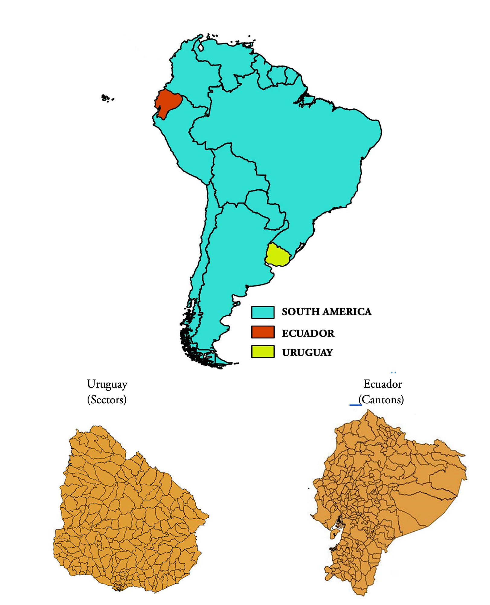
Source: INEC (National Institute of Statistics and Censuses) of Ecuador and INE (National Institute of Statistics) of Uruguay. Elaboration: the authors.
This paper follows the methodology proposed by Santos and Villatoro (2016) to build the MPI, but at a local level. We rely on this methodology because the authors develop an ad hoc Multidimensional Poverty Index for Latin America.
To formalize the indicator, let be the achievement in each dimension of each household i = 1, …, n in each canton/sector r = 1, …, R and j = 1,…, d be the dimensions of relative poverty to be explored. Let be the deprivation cut-off for poverty indicator j, and it is defined that when and otherwise. Then, the deprivation of each person is weighted by the indicator’s weight such that . Practically, the deprivation score is computed for each person as . We call this the first deprivation score indicator. There is a second cut-off for this score, denoted by k, to define relative poverty. Thus, a person is poor when . For each canton/sector r, following Santos and Villatoro (2016) we have
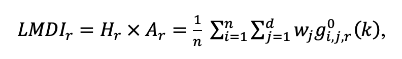
where LMPIr is the Local Multidimensional Poverty Index in region r, bounded by 0 (no poverty) and 1 (all households have the maximum level of deprivation); however, for the sake of simplicity the indicator has been rescaled to 100. LMPIr is the product of the sub-indices H and A, and it measures two things: the proportion of people who are multidimensionally poor in each canton/sector, Hr, (also called the poverty incidence), and the intensity given by the weighted average of deprivation among the poor, Ar. In more detail, Hr = q/n is the proportion of poor people in each administrative location, where is the number of households identified as poor, while Ai,r is the average intensity of deprivation among the poor, defined as . LMPIr is robust to dichotomizing individuals’ achievements into deprived and non-deprived. This means that poverty values do not change as a consequence of changes in the scales of the variables. Finally, the LMPIr allows a decomposition into sub-indices called censored headcount ratios, which depict the percentage of the population that is poor and deprived in dimension j.
The sources of information used are the national censuses of Ecuador and Uruguay, conducted in 1990 and 2010 and 1996 and 2011, respectively. The variables considered in the analysis are presented in Table 1. The indicator is constructed as a linear weighting index, where the variables are evenly weighted at 1/7 for each element of blocks A, B, and C, and subcomponents are consequently similarly weighted (Decacnq and Lugo, 2013). Block A refers to human capital and comprises education, block B captures housing characteristics and includes wall, roof, and floor materials, and block C describes access to public services (safe water, piped water, and electricity). The variables are dichotomous, so the deprivation cut-off identifies the presence or absence of a determined characteristic, as described in Table 1. The second cut-off k that determines whether a person is considered poor is set to over 2/7, meaning that a poor person is a household with more than two deprivation characteristics.[3]
The choice of indicators is based on the information available across censuses. In particular, we needed to have the same indicators for both countries and for both years considered. Moreover, our choice is guided by the literature focusing on deprivation indexes in Latin America, such as Obaco et al. (2020), Durán and Condorí (2017), and Cabrera-Barona et al. (2017). These studies consider that in exploring poverty, the minimum requirements that allow for comparability across countries are based on three blocks: education, housing materials, and access to public services. Finally, given the absence of information on income, we follow the Ministry of Housing, Communities & Local Government of the UK (2019), which considers as deprivation only the types of deprivation resulting from a low income that does not cover basic needs, excluding low income itself.
Table 1.
Variables used in the construction of the LMPI
| Block | Name | Variable | Weight |
| A | Education | 1 if the head of the household has a high school education or lower and 0 otherwise | 1/7 |
| B | Walls | 1 if the walls are not made of brick or stone and 0 otherwise | 1/7 |
| Roof | 1 if the roof is not made of concrete, zinc, or tiles and 0 otherwise | 1/7 | |
| Floor | 1 if the floor is not made of concrete, stone, brick, tiles, or parquet and 0 otherwise | 1/7 | |
| C | Safe water | 1 if the household has no access to safe public water and 0 otherwise | 1/7 |
| Piped water pipes | 1 if the water does not come from pipes at the house or close to it and 0 otherwise | 1/7 | |
| Electricity | 1 if the household does not have electricity and 0 otherwise | 1/7 |
Empirical Strategy
To explore the subnational dynamics of the LMPI, we rely on the so-called salter graph and on a spatial extension of the classical Markov transition matrix proposed by Rey (2001). In the salter graph, municipalities are first ranked according to their LMPI values, or its components as collected in the first census, and this is then plotted on the x-axis. Subsequently, holding the base-year rank positions of municipalities constant, the corresponding LMPI in the last census year considered is plotted. This allows us to visually identify changes in the relative position of a municipality with respect to itself in time and with respect to other municipalities in the same year.
The spatial extension of the Markov transition matrix is based on the standard Markov transition matrix. The latter follows a stochastic process where the result of each phase depends on the prior event, without considering the results before this step. Thus, each event has a finite number of possible results, and its associated probabilities are linked to the event immediately prior to it. If we have n periods, the process can be represented as follows:
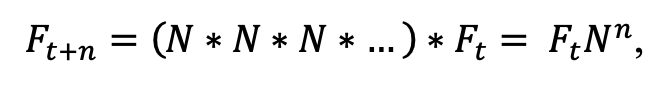
where the final distribution in the last period, is the result of the initial distribution multiplied by the transition probability matrix N to the power of n, where N has dimension and is the number of regions or observations analysed. The limiting transition probabilities of N are approximated to an ergodic or steady-state distribution vector, that is,
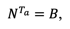
where B is the steady-state matrix for the system and is the number of years required to reach this steady state. Then, it is possible to compute the time to reach the steady state, , where N determines the properties of this long-run distribution.
The spatial extension of the transition matrix is based on Moran’s I (MI), which provides a spatial classification of the states in the distribution at one point in time. MI is defined as
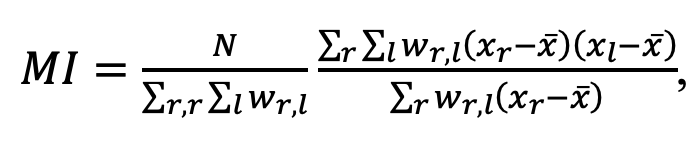
where r and l are the and the regions, the total number of which is R; x is the variable of interest; is its mean; and is an element of the row-standardized spatial weights matrix W, which is defined by means of queen criteria. When W is standardized by row, MI varies between –1 and 1. A significant positive coefficient points to positive spatial autocorrelation, i.e., clusters of areas with similar values are identified. The reverse indicates a negative association, and a non-significant value indicates the absence of spatial autocorrelation.
MI can be visualized in a Moran scatterplot, which relates a variable on the x-axis to its spatial lagged values on the y-axis. The Moran scatterplot has 4 quadrants (anticlockwise from the top right): in the first and third (high–high, HH, and low–low, LL, respectively), areas with high (low) values of a variable are surrounded by others with high (low) values, and in the second and fourth quadrants (low–high, LH, and high–low, HL, respectively), areas with low (high) values of a variable are surrounded by others with high (low) values. When regions are concentrated in the HH and LL quadrants, there are clusters of similar values, with a consequent positive spatial autocorrelation. The opposite happens if there is a negative spatial association, where the values are in the HL and LH quadrants.
The construction of the spatial transition matrix is based on the Moran scatterplots in the two years of analysis. After identifying the HH, HL, LH, and LL clusters for the two years, the spatial transition matrix is obtained from the frequencies of movement between quadrants between the two years.
Results
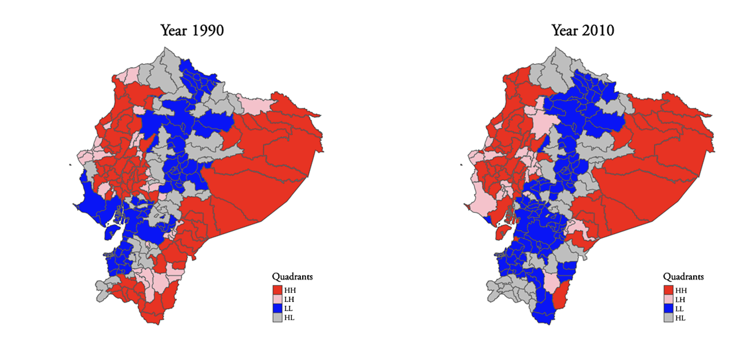
Figures 2 and 3 show the LMPI for Ecuador and Uruguay, respectively, in the two years of analysis. For both countries, the LMPI does not seem to vary randomly across space. In Ecuador, higher values are observed in the eastern part, namely the Coastal region, and in the western region, i.e., the Amazon region. In the Sierra region that crosses the center of the country from North to South, the LMPI shows lower values. Slight differences are observed between the two censuses, with the cantons in the Coastal and Amazon regions having higher values compared to other cantons in the same year.
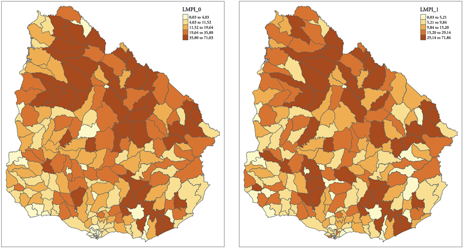
In Uruguay, sectors in the northern areas show higher LMPI values in both years. No particular changes can be appreciated in terms of spatial distribution between the two censuses.
Figure 2.
Maps of the LMPI for Ecuador in 1990 and 2010
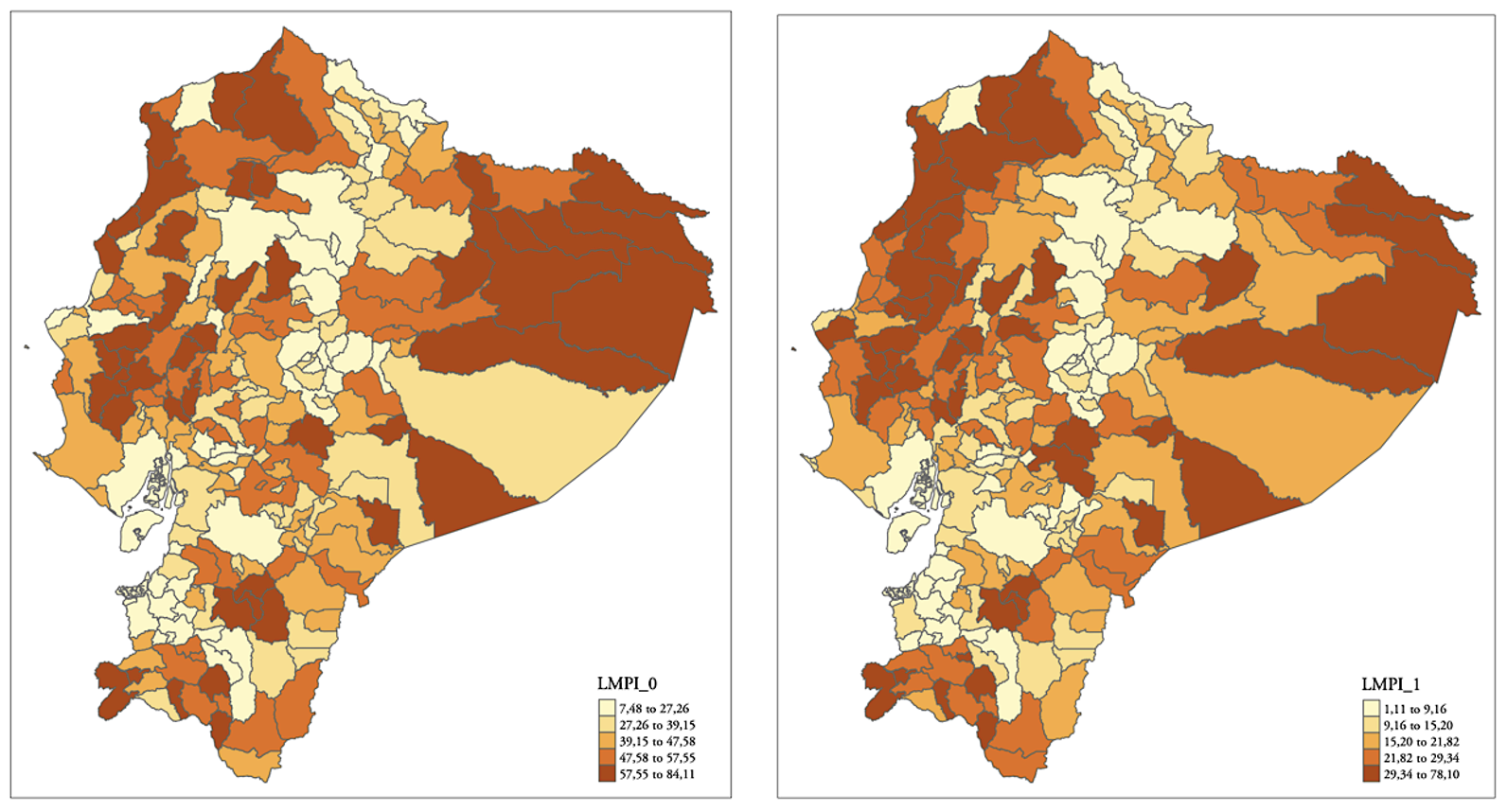
Figure 3.
Maps of the LMPI for Uruguay in 1995 and 2011
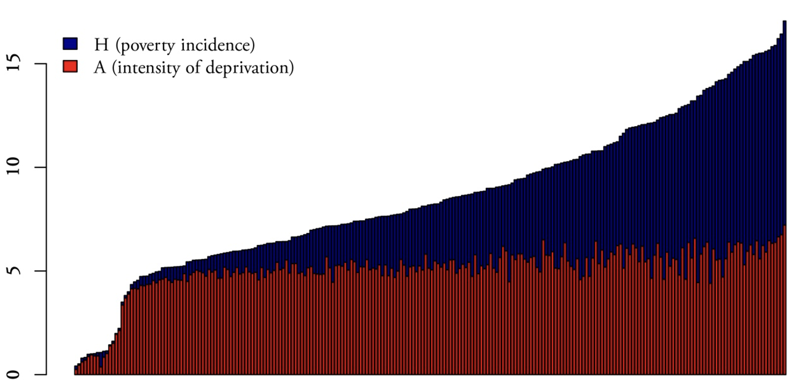
Figures 4 and 5 show the salter graphs for the LMPI and its components A and H, for Ecuador and Uruguay, respectively. The thin black dotted line interpolates the LMPI for later census, thus representing the trend in the later census.
In Ecuador (Figure 4 a), all but three cantons show a strong reduction in LMPI levels between the two periods. The dotted line indicates that the reduction is comparatively lower in cantons with lower initial values of the LMPI. As shown in Figure A1 in Appendix A, the reduction in LMPI is led by the reduction of component H, poverty incidence, while component A, the intensity of deprivation, is quite stable over time. The correlation between the growth of the LMPI and of component A is equal to –0.13, and that between the growth of the LMPI and of component H is equal to 0.98. The salter graphs for components A and H (Figure 4b and c) show that the level of the first decreased slightly between the 1990 and 2010 censuses, with a higher frequency of downward movements at the high end of the distribution. Component H, on the other hand, shows a generally strong reduction and, contextually, a low persistence in ranking position, denoting a change in poverty incidence among municipalities. Furthermore, in various cases at the top of the distribution poverty incidence levels in 2010 are close to those in 1990.
Regarding Uruguay, Figure 5a shows that the LMPI did change across sectors, as 40% had a higher LMPI in 2011 than in 1996. The frequency of downward movements in the distribution is higher at the middle and high end of the distribution, while in the low end a consistent number of sectors show upward movements. In Figure A2 in Appendix A, we can observe that neither component A nor H particularly change in terms of values in the two censuses. The correlation between the increase in the LMPI and the growth of component A is equal to 0.18, and that between the increase in the LMPI and the growth of component H is equal to 0.61.
In Figure 5b, it is interesting to note how the intensity of deprivation (component A) grew for sectors at the bottom end of the distribution, but not for the rest. Figure 5c, finally, shows that the poverty incidence (component H) has a pattern similar to that in Figure 5a, with the levels of sectors ranked at the top end of the distribution decreasing and the levels of sectors at the bottom end of the distribution generally growing.
Figure 4.
Salter graph for Ecuador
a) LMPI
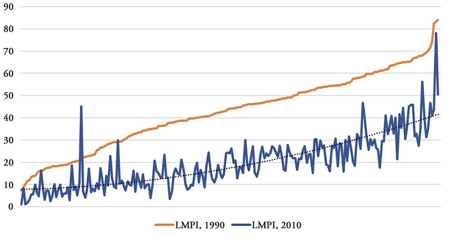
Note: The dotted line represents the trendline.
b) Component A
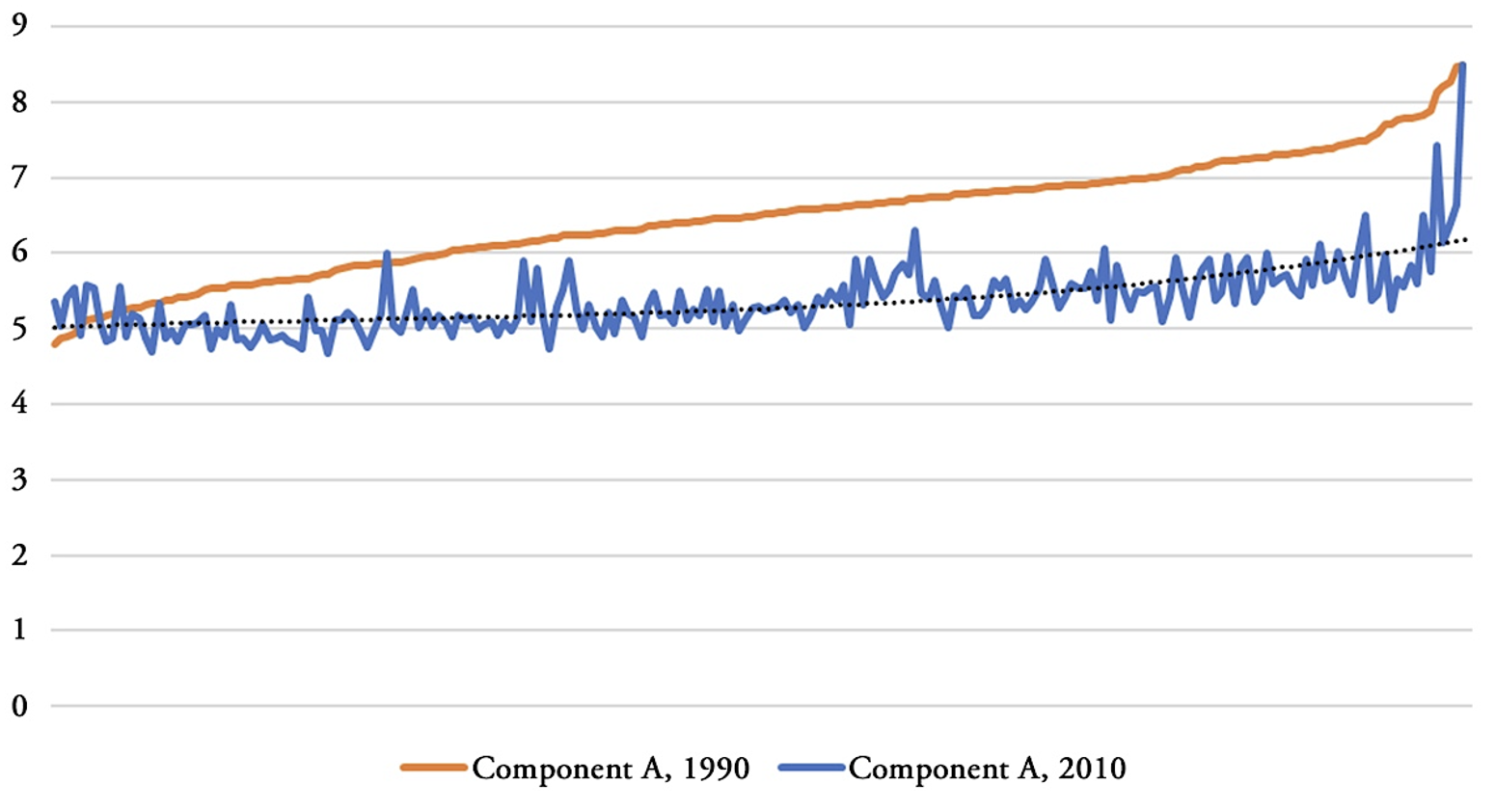
Note: The dotted line represents the trendline.
Salter graph for Ecuador
c) Component H
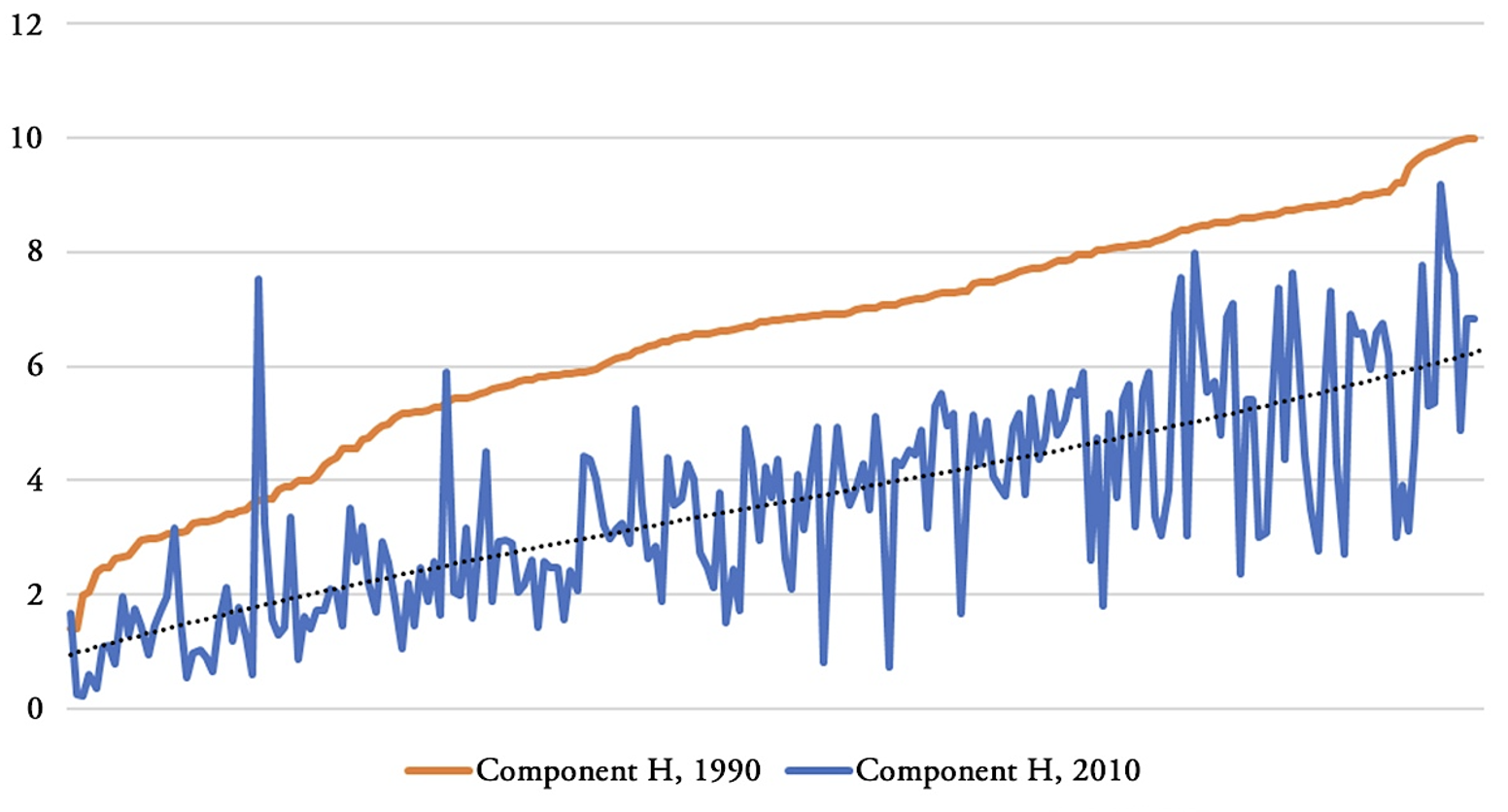
Note: The dotted line represents the trendline.
Figure 5.
Salter graph for Uruguay
a) LMPI
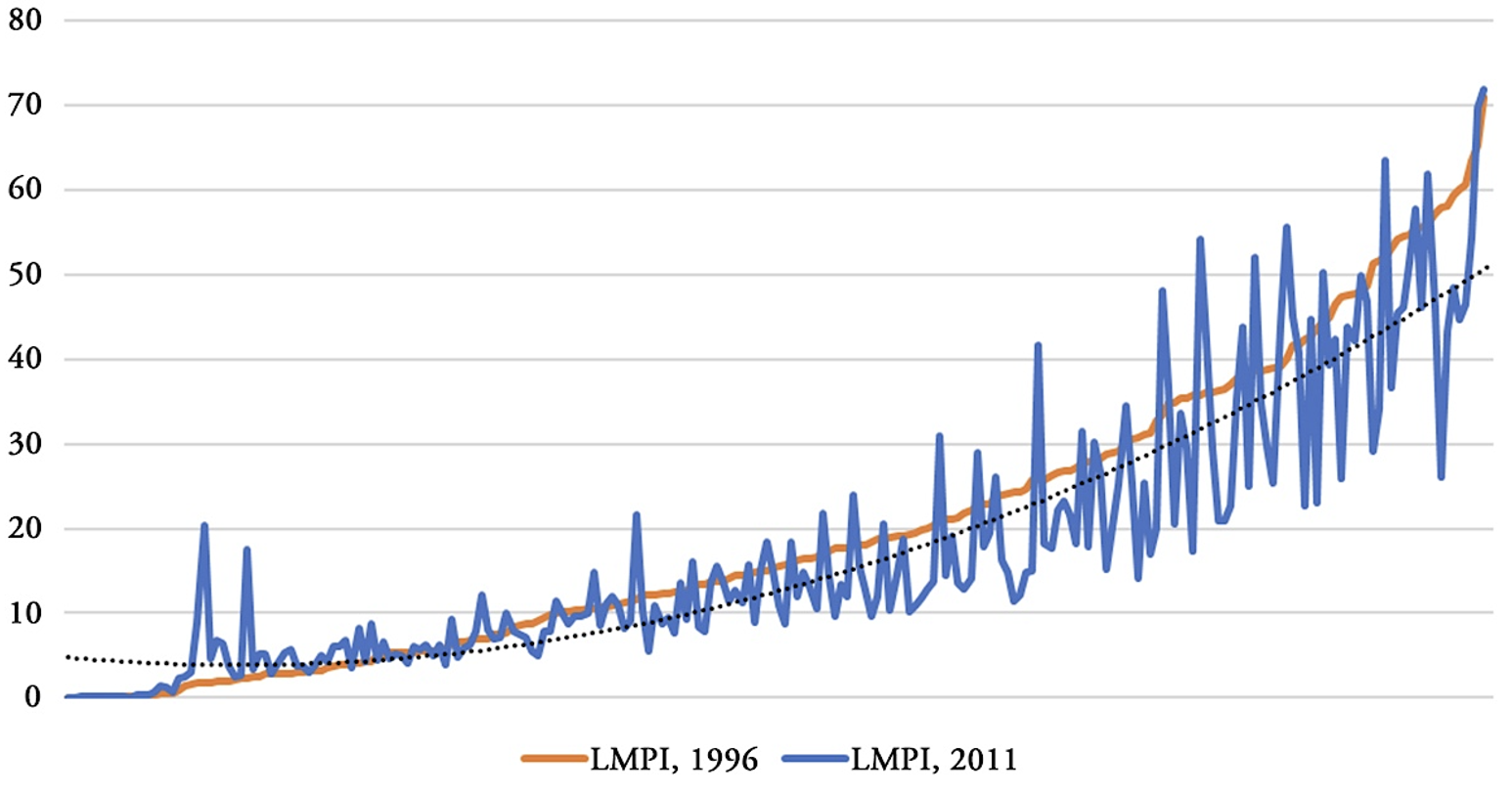
Note: The dotted line represents the trendline.
b) Component A

Note: The dotted line represents the trendline.
c) Component H
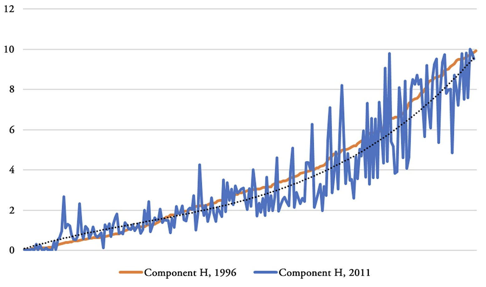
Note: The dotted line represents the trendline.
In Table 2, the descriptive statistics for the LMPI and its components for Ecuador and Uruguay confirm some of the intuitions stemming from the previous maps and graphs. Regarding Ecuador, at the canton level the LMPI almost halved between the 1990 and 2010 censuses (from 43 to 20, on average). The variability decreased as well, as did the maximum and minimum values. Moran’s I, which is used to check for the presence of spatial autocorrelation, is positive and statistically significant for both years, highlighting the presence of clusters of cantons with similar values of the LMPI located close to each other. Regarding the components of the LMPI, the mean, minimum, maximum, and standard deviation of the intensity of deprivation, A, decreased only slightly in the second year, while component H, i.e., the proportion of multidimensionally poor, presents a strong reduction in the mean and minimum values, while the maximum and standard deviation almost do not vary. It is worth mentioning that a positive and statistically significant spatial autocorrelation is observed for both A and H in both years. Finally, on average, LMPI growth is negative, as is the growth of components A and H, and MI is always significant and between 0.35 and 0.39.
Regarding Uruguay, at a sector level the LMPI decreased slightly (on average, from 20 to around 18). The minimum and maximum values remained almost the same, and the standard deviation also decreased. Component A, the intensity component, increased slightly, as did the minimum and maximum values, while the standard deviation decreased. The proportion of poor, H, decreased slightly, on average, as did the standard deviation. For all components, we observe positive and significant spatial autocorrelation that is constant over time. Finally, the average growth of the LMPI is equal to –0.002 and is mainly due to the variation in H. MI is significantly different from zero for both the growth of the LMPI and that of A and H.
Table 2.
Results for the LMPI and its components, averaged for each sample
| Ecuador | |||||||
| Variable | Obs. | Mean | Std. Dev. | Min. | Max. | Moran’s I | |
| 1990 | LMPI | 217 | 42,71 | 16,36 | 7,48 | 84,11 | 0,390*** |
| A | 217 | 6,47 | 0,75 | 4,80 | 8,48 | 0,450*** | |
| H | 217 | 6,47 | 2,04 | 1,39 | 9,98 | 0,345*** | |
| 2010 | LMPI | 217 | 19,84 | 11,93 | 1,11 | 78,09 | 0, 436*** |
| A | 217 | 5,37 | 0,45 | 4,66 | 8,49 | 0,480*** | |
| H | 217 | 3,59 | 1,89 | 0,23 | 9,20 | 0,451*** | |
| LMPI growth | 217 | -0,044 | 0,020 | -0,118 | 0,037 | 0,380*** | |
| A growth | 217 | -0,009 | 0,004 | -0,012 | 0,006 | 0,359*** | |
| H growth | 217 | -0,035 | 0,022 | -0,114 | 0,036 | 0,392*** | |
| Uruguay | |||||||
| Variable | Obs. | Mean | Std. Dev. | Min. | Max. | Moran’s I | |
| 1996 | LMPI | 230 | 19,97 | 17,11 | 0,02 | 71,03 | 0,376*** |
| A | 230 | 5,02 | 1,23 | 0,25 | 7,22 | 0,919*** | |
| H | 230 | 3,59 | 2,85 | 0,03 | 9,91 | 0,360*** | |
| 2011 | LMPI | 230 | 17,64 | 15,61 | 0,028 | 71,86 | 0,230*** |
| A | 230 | 5,24 | 0,62 | 4,29 | 8,18 | 0,348*** | |
| H | 230 | 3,31 | 2,73 | 0,00 | 2,72 | 0,224*** | |
| LMPI growth | 230 | -0,002 | 0,032 | -0,089 | 0,163 | 0,420*** | |
| A growth | 230 | 0,007 | 0,035 | -0,018 | 0,256 | 0,946*** | |
| H growth | 230 | -0,009 | 0,043 | -0,241 | 0,126 | 0,695*** | |
Note: ∗p < 0,1; ∗∗p < 0,05; ∗∗∗p < 0,01.
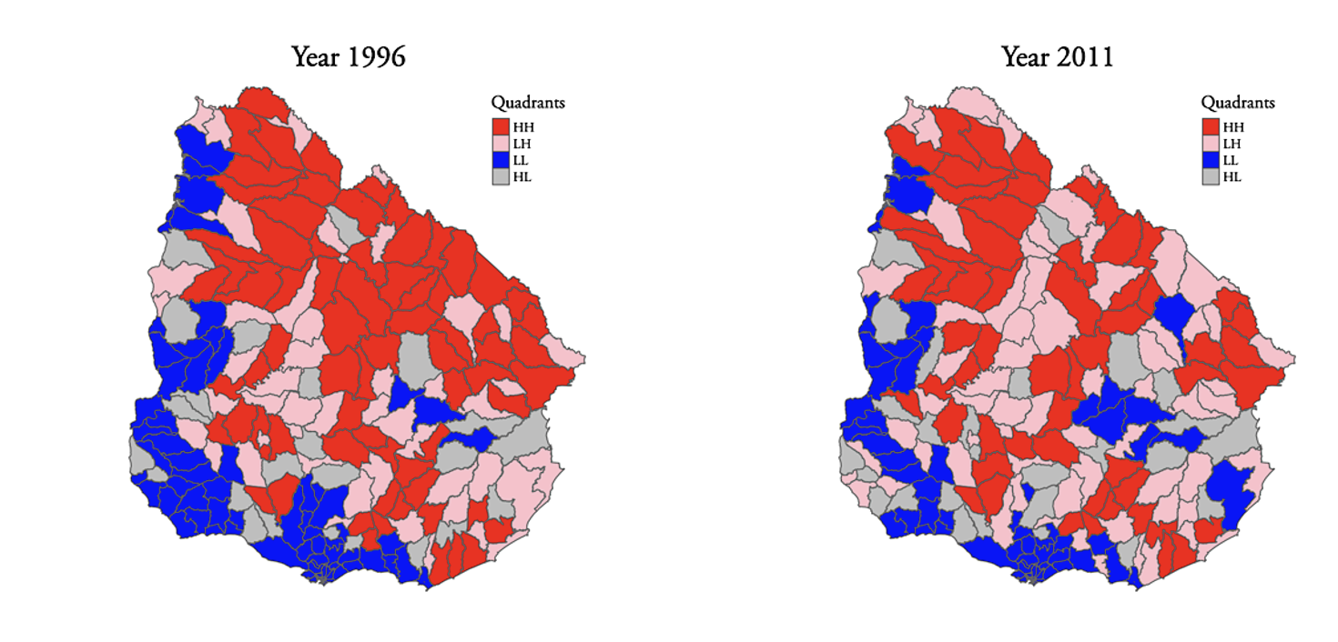
Based on the Moran scatterplots reported in Appendix A (Figures A3 to A6), we construct the spatial transition matrix for the two countries to analyze spatial dynamics between the two censuses in the two countries. In Tables 3 and 4, we observe the spatial transition probability matrices for Ecuador and Uruguay, respectively. The ergodic transition matrix is presented below the transition probability matrix. Results are presented for the LMPI, component A, and component H, as before.
Table 3.
Spatial transition and transition probability matrix for Ecuador
a) LMPI
| Transition probability matrix | Frequency of cantons in T=0 | HH | LH | LL | HL |
| HH | 78 | 0,76 | 0,06 | 0,08 | 0,10 |
| LH | 32 | 0,16 | 0,63 | 0,22 | 0,00 |
| LL | 73 | 0,00 | 0,04 | 0,93 | 0,03 |
| HL | 34 | 0,12 | 0,03 | 0,29 | 0,56 |
| Ergodic | 0,10 | 0,10 | 0,73 | 0,07 |
b) A
| Transition probability matrix | Frequency of cantons in T=0 | HH | LH | LL | HL |
| HH | 84 | 0,64 | 0,12 | 0,09 | 0,14 |
| LH | 30 | 0,20 | 0,33 | 0,43 | 0,03 |
| LL | 74 | 0,09 | 0,08 | 0,80 | 0,03 |
| HL | 29 | 0,14 | 0,00 | 0,55 | 0,31 |
| Ergodic | 0,24 | 0,11 | 0,57 | 0,08 |
b) H
| Transition probability matrix | Frequency of cantons in T=0 | HH | LH | LL | HL |
| HH | 78 | 0,80 | 0,11 | 0,08 | 0,10 |
| LH | 33 | 0,18 | 0,57 | 0,21 | 0,03 |
| LL | 60 | 0,02 | 0,05 | 0,92 | 0,02 |
| HL | 46 | 0,17 | 0,04 | 0,32 | 0,46 |
| Ergodic | 0,15 | 0,12 | 0,67 | 0,05 |
Table 4.
Spatial transition matrix for Uruguay
a) LMPI
| Transition probability matrix | Frequency of cantons in T=0 | HH | LH | LL | HL |
| HH | 66 | 0,70 | 0,21 | 0,01 | 0,08 |
| LH | 41 | 0,00 | 0,93 | 0,07 | 0,00 |
| LL | 98 | 0,02 | 0,10 | 0,82 | 0,06 |
| HL | 25 | 0,12 | 0,04 | 0,00 | 0,84 |
| Ergodic | 0,06 | 0,58 | 0,23 | 0,12 |
b) A
| Transition probability matrix | Frequency of cantons in T=0 | HH | LH | LL | HL |
| HH | 132 | 0,40 | 0,14 | 0,39 | 0,07 |
| LH | 39 | 0,13 | 0,08 | 0,74 | 0,05 |
| LL | 48 | 0,31 | 0,27 | 0,33 | 0,08 |
| HL | 11 | 0,00 | 0,00 | 0,82 | 0,18 |
| Ergodic | 0,28 | 0,18 | 0,46 | 0,08 |
b) H
| Transition probability matrix | Frequency of cantons in T=0 | HH | LH | LL | HL |
| HH | 71 | 0,70 | 0,22 | 0,01 | 0,06 |
| LH | 49 | 0,00 | 0,90 | 0,10 | 0,00 |
| LL | 86 | 0,02 | 0,09 | 0,84 | 0,05 |
| HL | 24 | 0,21 | 0,00 | 0,04 | 0,75 |
| Ergodic | 0,08 | 0,49 | 0,33 | 0,08 |
Regarding Ecuador (Table 3), 78 cantons were classed in the HH quadrant in 1990 and, of those, 76% remained in the same quadrant in 2010. The remainder were equally distributed across the other quadrants. Regarding the 73 cantons classed in the LL quadrant, 93% remained in the same one in 2010, and of the 32 cantons initially in quadrant LH, around half did not change quadrant while 29% shifted to quadrant LL and 16% to HH. Finally, of the 34 cantons that were in quadrant HL, 56% remained in that quadrant and 29% moved to quadrant LL. Overall, we can say that there is a high probability of persistence of cantons with a high (low) LMPI being surrounded by others with a high (low) LMPI. When we observe the ergodic probability interacted for 1000 years, we find 73% of cantons in quadrant LL and the remaining distributed almost evenly between the other quadrants. This means that in the long run, the country would have half of its cantons with an LMPI below the average surrounded by others with an LMPI below the average.
Regarding Uruguay (Table 4), of the 98 sectors in the LL quadrant in 1996, 82% remained in the same quadrant in 2011, while 10% moved to quadrant LH. As for the 66 sectors in quadrant HH in 1996, 21% moved to quadrant LH in 2011 and 70% remained in the same quadrant. With respect to the 41 sectors in the LH quadrant in T0, 93% remained in the same quadrant and 7% moved to the LL quadrant. The path of the spatial transition probability matrix for component H is similar to that of the LMPI, while that of component A is slightly different, generally with a higher likelihood of transition toward the HH quadrant. The ergodic distribution, however, shows 57% of cantons in the LL quadrant and 24% in the HH quadrant.
Finally, regarding the 25 sectors in the HL quadrant in T0, 84% remained in the HL quadrat and 12% moved to the HH quadrant in 2011. Overall, for Uruguay as well we observe a high degree of persistence across quadrants, and sectors that do move tend to become LH sectors. Regarding the ergodic distribution, in the long run we observe a probability of 58% that sectors belong to quadrant LH. Component H shows close similarities to the LMPI. Component A shows very little persistence, with a high share of sectors moving toward quadrant HH.
Conclusions and policy implications
In this paper, we apply the MPI indicator of Santos and Villatoro (2016) at the municipal level to assess spatial dynamics and evolution over time, using data from the 1990 and 2010 censuses for Ecuador and the 1996 and 2011 censuses for Uruguay. Our results add to the information available regarding Ecuador and provide some additional data regarding Uruguay, a country for which there is a dearth of information. This contribution is even more significant when we consider that the MPI is composed of two parts, the incidence of poverty (H) and the intensity of deprivation (A), which offer further insights on the characteristics of multidimensional poverty in the two countries. To build the MPI at the local level, we constructed the Local Multidimensional Poverty Index (LMPI) using nine variables related to basic infrastructure, public services, and housing materials.
In carrying out our analysis, we employ a mix of techniques, namely salter graphs, Moran’s I, Moran scatterplots, and spatial transition matrices, which allow us to shed light on various aspects of the spatial and temporal dynamics of the LMPI.
The results show that the LMPI is generally lower for Uruguay than for Ecuador. In the latter country, however, a strong improvement is observed, with multidimensional poverty levels halving between 1990 and 2010 and almost reaching the levels of Uruguay, where the LMPI barely changed between the two years investigated. The reduction in Ecuador is mainly led by an improvement in poverty incidence H, whereas the intensity of deprivation A decreases only slightly.
The spatial dynamics, accounted for by Moran’s I, Moran scatterplots, and the spatial transition probability matrices, indicate that a significant positive spatial autocorrelation is present. Indeed, depending on the indicator, the period, and the country, between 60% and 78% of municipalities fall into the high–high (HH) or low–low (LL) quadrants. This means that a large majority of municipalities are surrounded by others with similar values of the indicator under analysis. In Ecuador, a certain degree of spatial persistence is observed for quadrants HH and LL, while administrative areas belonging to the remaining quadrants (HL and LH) in the first period tend to shift to the HH quadrant. This is confirmed in the long run by the ergodic distribution. Regarding Uruguay, high persistence is observed in all quadrants, especially for the LMPI and component H. Surprisingly, sectors tend to move to the LH quadrant, and this is a confirmed equilibrium in the long run. Component A shows very little persistence, and sectors tend to move to quadrant LL and, to a lesser extent, quadrant HH.
This evidence has various policy implications for Ecuador and Uruguay. First, both countries need to reinforce territorial cohesion and focus on reducing the LMPI in a balanced way, i.e., without creating spatial clusters of poverty due to subnational gaps in the implementation of poverty-reduction policies. To reach this aim, we suggest promoting regional, local, and place-based policies that allow a particular focus on specific areas within each country. The analysis of dedicated policies, however, is beyond the scope of this paper. Second, the simple local index of multidimensional poverty we propose can be used by policymakers as a tool to establish and measure goals at a local level and monitor differences among areas and clusters both in a given year and over time. This would allow detecting those areas that show improvement and the successful policies put into action. The identification of best practices could then contribute to balancing territory inequalities.
Summing up, we consider the LMPI to be an important tool to reach several Sustainable Development Goals (SDGs) in developing economies, especially those related to poverty, education, inequality, and well-being at the subnational level. This index can be easily updated with upcoming censuses, and an analysis using more recent data will show whether the trends presented in our paper have been maintained or have changed.
Finally, regarding avenues for future research, we consider it important to understand which local factors influenced the observed changes in the LMPI. In addition, due to the relative simplicity of the index, it would be feasible to consider more countries in Latin America or to explore the LMPI by subgroups of people based on gender, ethnicities, and age.
APPENDICES
Appendix A
Figure A1.
A and H components for Ecuador
a) 1990

b) 2010
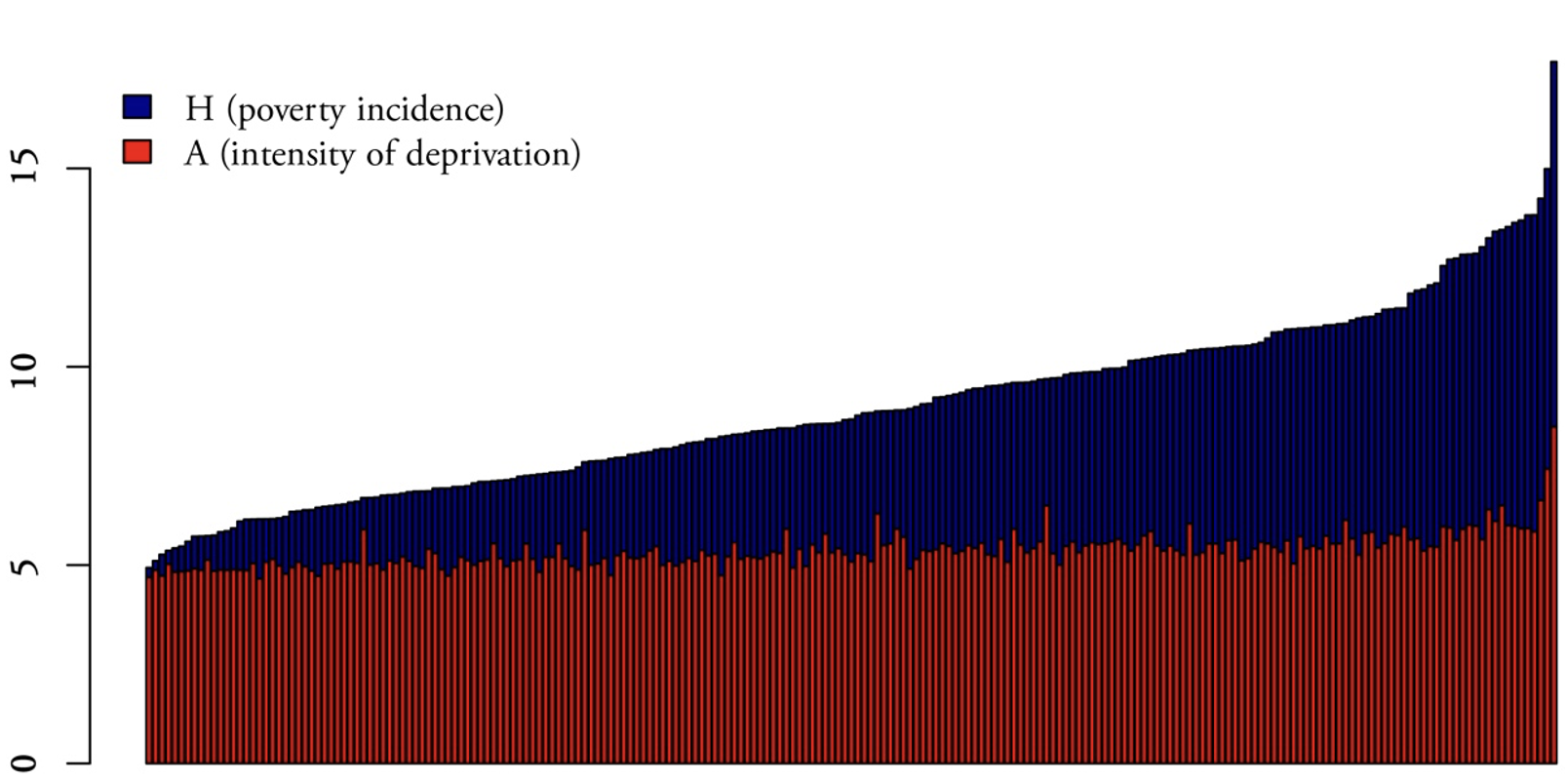
Figure A2.
A and H components for Uruguay
a) 1996
b) 2011

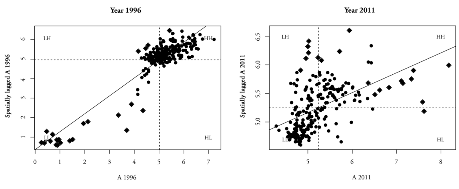
Figure A3.
Moran scatterplot for Ecuador
a) LMPI
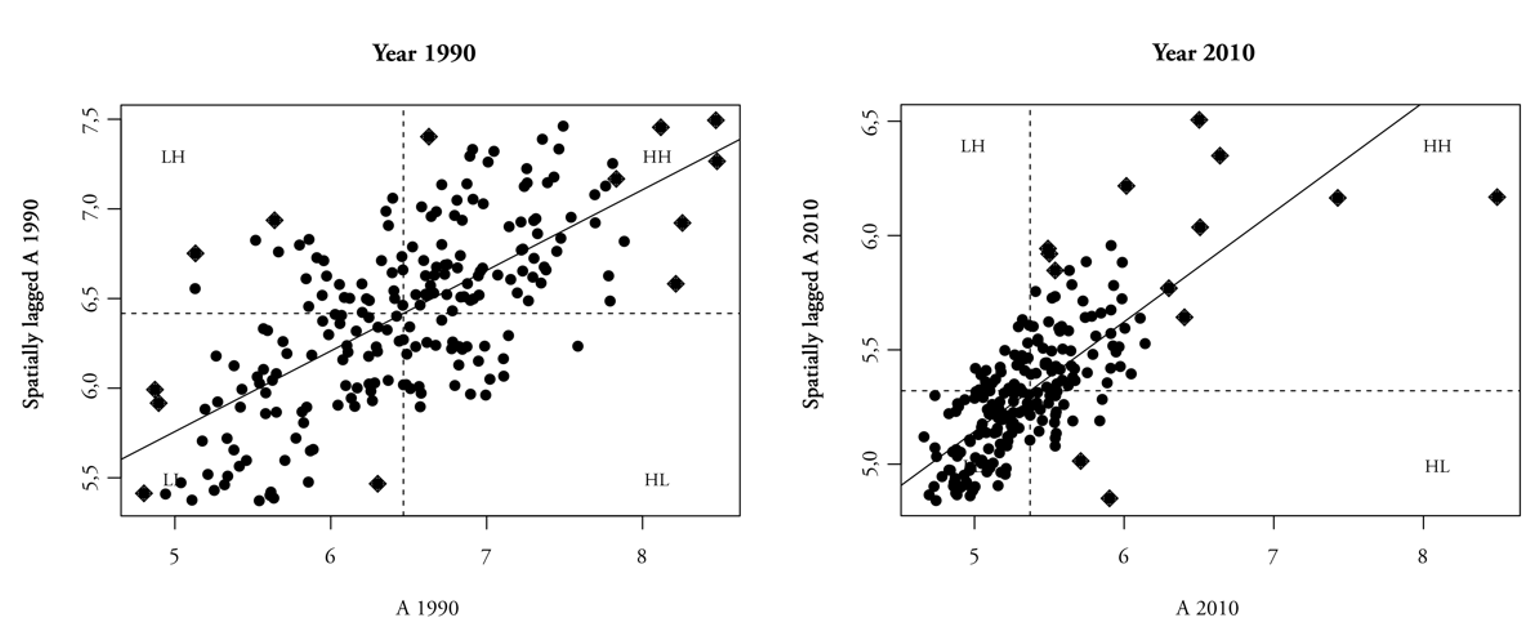
b) A

c) H
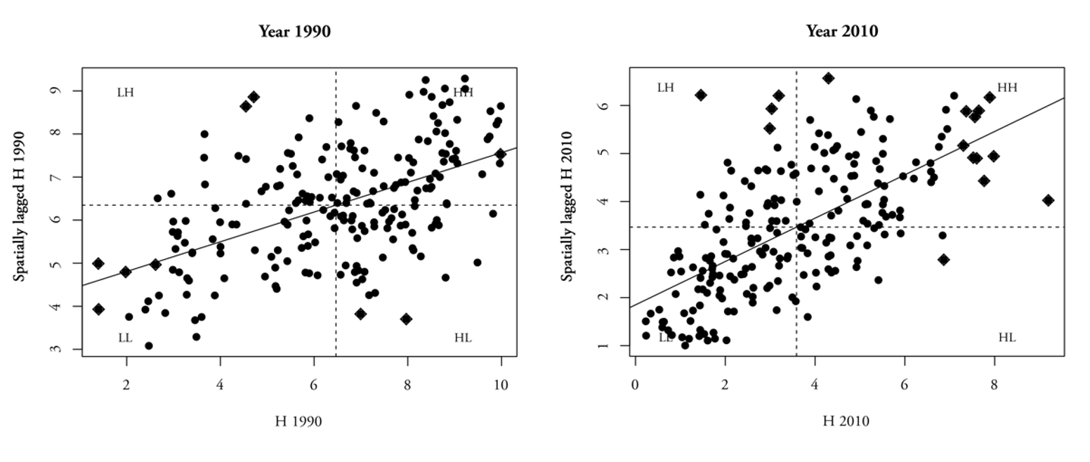
Figure A4.
Moran scatterplot map for Ecuador
a) LMPI
b) A

c) H
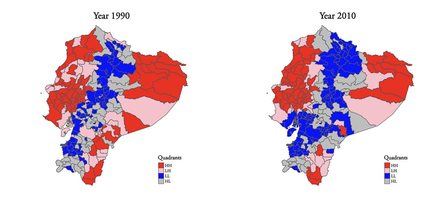
Figure A5.
Moran scatterplot for Uruguay
a) LMPI

b) A
c) H
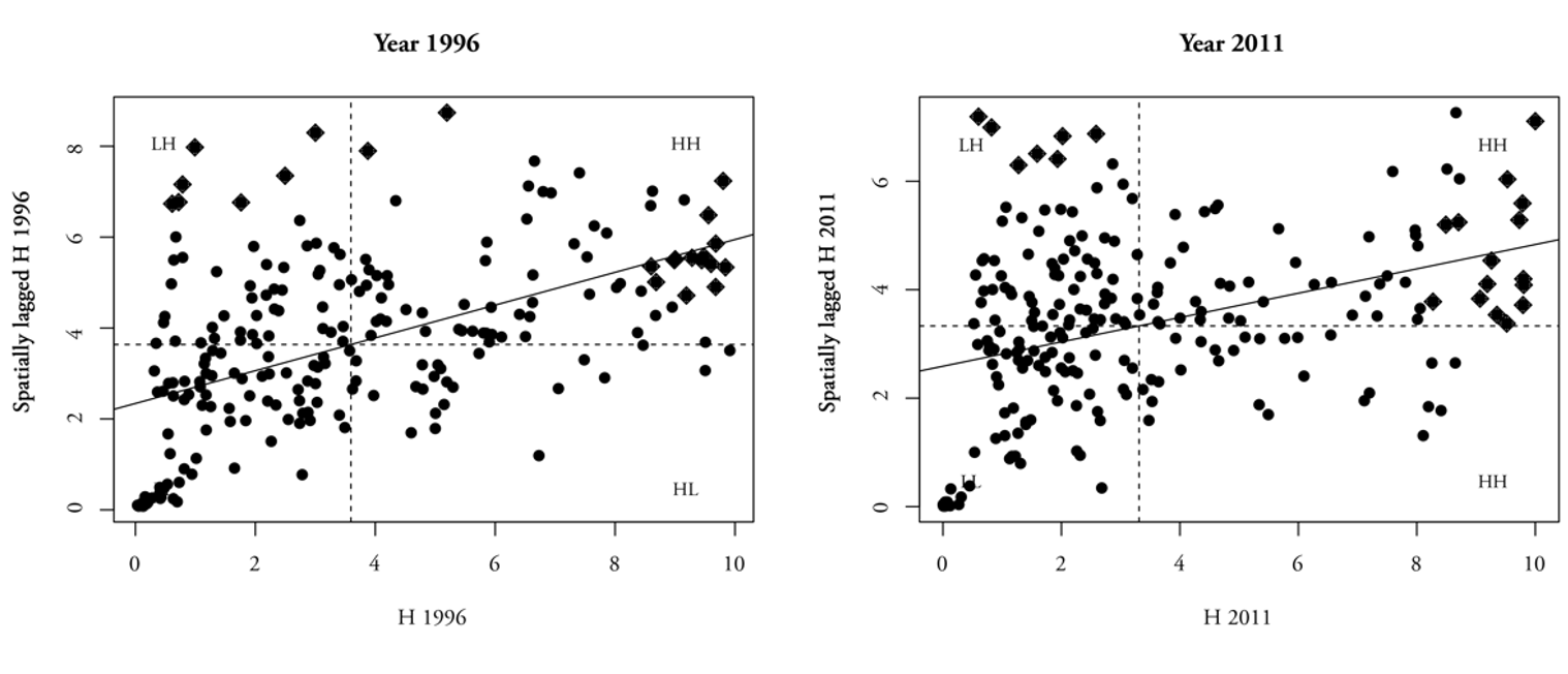
Figure A6.
Moran scatterplot map for Uruguay
a) LMPI
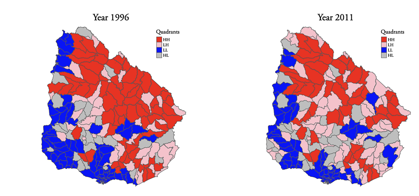
b) A
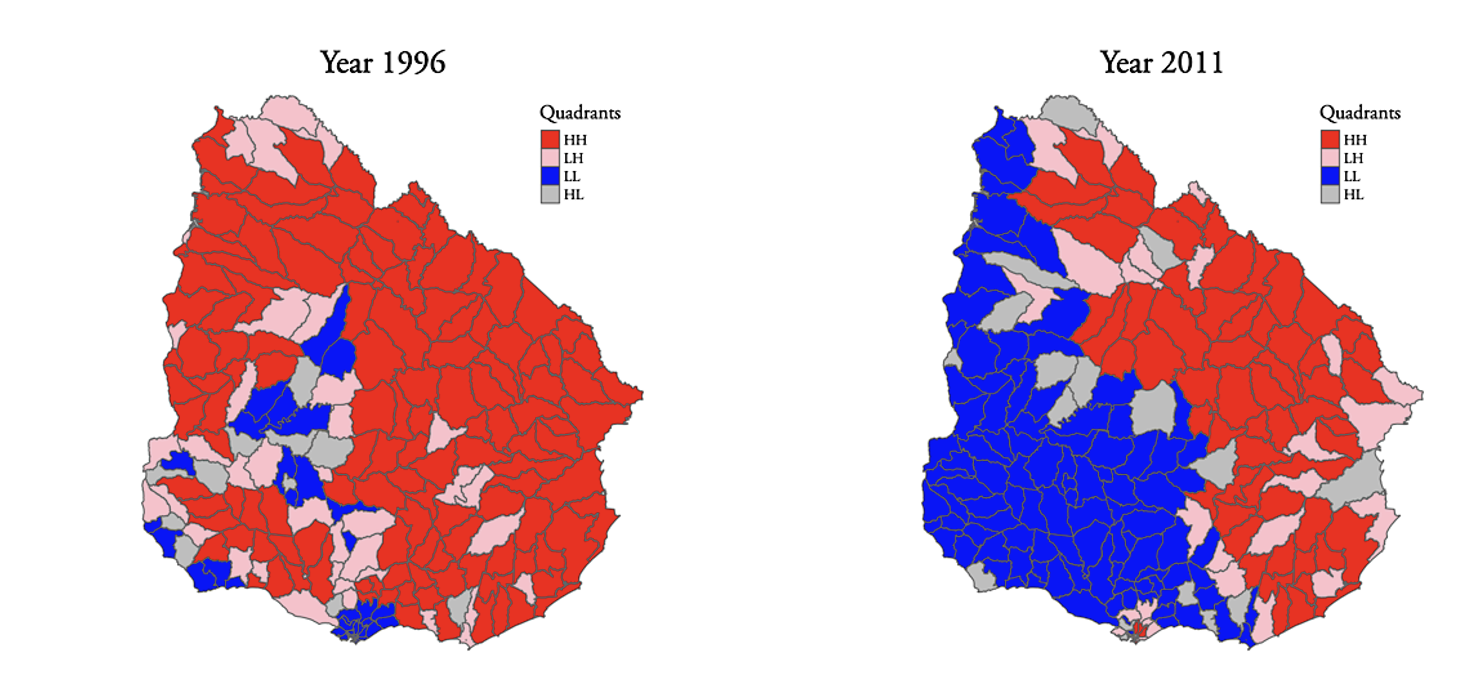
c) H
References
Alkire, S., Foster, J. E., Seth, S., Santos, M. E., Roche, J. M., & Ballon, P. (2015). Multidimensional Poverty Measurement and Analysis. Oxford University Press, Ch. 4. https://ophi.org.uk/multidimensional-poverty-measurement-and-analysis-contents/
Alkire, S., Kanagaratnam, U., & Suppa, N. (2020). The global Multidimensional Poverty Index (MPI) 2020. OPHI MPI Methodological Note 49, Oxford Poverty and Human Development Initiative, University of Oxford. http://hdr.undp.org/en/2020-MPI
Alkire, S., Roche, J. M., & Seth, S. (2011). Sub-national Disparities and Inter-temporal Evolution of Multidimensional Poverty across Developing Countries, OPHI Research in Progress N° 32ª. https://www.ophi.org.uk/wp-content/uploads/OPHI-RP-32a-2011.pdf
Alkire, S., Roche, J. M., & Vaz, A. (2017). Changes Over Time in Multidimensional Poverty: Methodology and Results for 34 countries. World Development, 94, 232–249. https://doi.org/10.1016/j.worlddev.2017.01.011
Alkire, S., & Santon, M. E. (2014). Measuring Acute Poverty in the Developing World: Robustness and Scope of the Multidimensional Poverty Index. World Development, 59, 251–274. https://doi.org/10.1016/j.worlddev.2014.01.026
Alkire, S., & Seth, S. (2015). Multidimensional Poverty Reduction in India between 1999 and 2006: Where and How? World Development, 72, 93–108. https://www.sciencedirect.com/science/article/abs/pii/S0305750X1500042X
Awasthi, A., Pandey, C. M., & Phil, M. (2017). Trends, prospects and deprivation index of disability in India: Evidences from census 2001 and 2011. Disability and Health Journal, 10, 247–256. https://doi.org/10.1016/j.dhjo.2016.10.011
Balen, J., McManus, D. P., Li, Y.-S., Zhao, Z.-Y., Yuan, L.-P., Utzinger, J., Williams, G. M. Li, Y., Ren, M.-Y., Liu, Z.-C., Zhou, J., & Raso, G. (2010). Comparison of two approaches for measuring household wealth via an asset-based index in rural and peri-urban settings of Hunan province, China. Emerging Themes in Epidemiology, 7(1), 17. ISSN 1742-7622. https://doi.org/10.1186/1742-7622-7-7
Booysen, F. Van der Berg S., & Burger, R. (2008). Using an Asset Index to Assess Trends in Poverty in Seven Sub-Saharan African Countries. World Development, 36, 1113–1130. https://doi.org/10.1016/j.worlddev.2007.10.008
Brueckner, J. K. (2013). Slums in developing countries: New evidence for Indonesia. Journal of Housing Economics, 22(4), 278–290. https://doi.org/10.1016/j.jhe.2013.08.001
Cabrera-Barona, P., Wei, C., & Hagenlocher, M. (2016). Multiscale evaluation of an urban deprivation index: Implications for quality of life and healthcare accessibility planning. Applied Geography, 70, 1–10. https://doi.org/10.1016/j.apgeog.2016.02.009
Carstairs, V., & Morris, R. (1989). Deprivation and mortality: an alternative to social class? J. Public Health, 11, 210–219. https://doi.org/10.1093/oxfordjournals.pubmed.a042469
Anda, D., Nathalie, G., Nobuaki H., Yudai H., Hiroyuki H., Murray L., Elnari P., Muna S. (2018). Spatial poverty and inequality in South Africa: A municipality level analysis. Southern Africa Labour and Development Research Unit. SALDRU Working Paper N° 221. https://ideas.repec.org/p/avg/wpaper/en8253.html
Decancq, K. & Lugo, M. A. (2013). Weights in multidimensional indices of wellbeing: an overview. Econometics Review, 32, 7–34. https://doi.org/10.1080/07474938.2012.690641
Durán, R. J. & Condorí, M. Á. (2017). Deprivation index for small areas based on census data in Argentina. Social Indicators Research, 89, 1–33. https://doi.org/10.1007/s11205-017-1827-6
Galiani, S., Gertler, P. J., Undurraga, R., Cooper, R., Martínez, S., & Ross, A. (2017). Shelter from the storm: Upgrading housing infrastructure in Latin America slums. Journal of Urban Economics, 98, 187–213. https://www.nber.org/papers/w19322
Gonzáles, C., Houweling, T., & Marmot, M. (2010). Comparison of physical, public and human assets as determinants of socioeconomic inequalities in contraceptive use in Colombia - moving beyond the household wealth index. International Journal for Equity in Health, 9, 9-12. https://doi.org/10.1186/1475-9276-9-10
Gómez-Salcedo, M. S., Galvis-Aponte, L. A. & Royuela, V. (2016). Quality of Work Life in Colombia: A Multidimensional Fuzzy Indicator. Social Indicators Research, 30(3), 911–936. https://doi.org/10.1007/s11205-015-1226-9
Havard, S., Deguen, S., Bodin, J., Louis, K., Laurent, O., & Bard, D. (2008). A small-area index of socioeconomic deprivation to capture health inequalities in France. Social Science & Medicine, 67, 2007–2016. https://doi.org/10.1016/j.socscimed.2008.09.031
Jarman, B. (1983). Identification of underprivileged areas, British Medical Journal (Clinical Research Ed.), 286, 1705–1709. https://doi.org/10.1136/bmj.286.6379.1705
Jimenez, J. & Alvarado, R. (2018). Efecto de la productividad laboral y del capital humano en la pobreza regional en Ecuador. Journal of Regional Research, 40, 141 a 165
Khadr, Z., Nour el Dein, M., & Hamed, R. (2010). Using GIS in constructing area-based physical deprivation index in Cairo Governorate, Egypt. Habitat International, 34, 264–272. http://dx.doi.org/10.1016/j.habitatint.2009.11.001
Lalloué, B., Monnez, J-M., Padilla, C., Hihal, W., Le Meur, N., Zmirou-Navier, D., & Deguen, S. (2013). A statistical procedure to create a neighborhood socioeconomic index for health inequalities Analysis. International Journal for Equity in Health, 12, 12–21. https://doi.org/10.1186/1475-9276-12-21
Machado, A. F., Golgher, A. B., & Antigo, M. F. (2014). Deprivation viewed from a multidimensional perspective: The case of Brazil. Cepal Review, 112, 125–146. http://hdl.handle.net/11362/37024
Mero-Figueroa, M., Galdeano-Gómez, E., Piedra-Muñoz, L., & Obaco, M. (2020). Measuring Well-Being: A Buen Vivir (Living Well) Indicator for Ecuador. Social Indicators Research, 152, 265–287. https://doi.org/10.1007/s11205-020-02434-4
OECD (2008). Handbook on Constructing Composite Indicators: Methodology and User Guide – ISBN 978-92-64-04345-9 Paris: OECD Publishing. https://www.oecd.org/els/soc/handbookonconstructingcompositeindicatorsmethodologyanduserguide.htm
Obaco, M., Royuela, V., & Matano, A. (2020). On the link between material deprivation and city size: Ecuador as a case study. Land Use Policy, 13 June, 104761. https://doi.org/10.1016/j.landusepol.2020.104761
Pasha, A. (2017). Regional Perspectives on the Multidimentional Poverty Index. World Development, 94, 268–285. https://doi.org/10.1016/j.worlddev.2017.01.013
Podova, D., & Pishniak, A. (2017). Measuring Individual Material Well-Being Using Multidimensional Indices: An Application Using the Gender and Generation Survey for Russia. Social Indicators Research, 130, 883–910. https://doi.org/10.1007/s11205-016-1231-7
Rey, S. (2001). Spatial Empirics for Economic Growth and Convergence. Geographical Analysis, 33(3), 195–214. https://doi.org/10.1111/j.1538-4632.2001.tb00444.x
Sánchez-Cantalejo, C., Ocana-Riola, R., & Fernández-Ajuria, A. (2008). Deprivation index for small areas in Spain. Social Indicators Research, 89, 259–273. https://doi.org/10.1007/s11205-007-9114-6
Santos, M. A., & Villatoro, P. (2018). A Multidimensional Poverty Index for Latin America. The Review of Income and Wealth, 64, 52–82. https://www.ophi.org.uk/wp-content/uploads/OPHIWP079.pdf
Teixeira Costa, G. O., Machado, A. F., & Amaral, P. V. (2018). Vulnerability to poverty in Brazilian municipalities in 2000 and 2010: A multidimensional approach. Economía, 19, 132-148. https://doi.org/10.1016/j.econ.2017.11.001
Townsend, P., Phillimore, P., & Beattie, A. (1988). Health and deprivation: inequality and the North, London: Routledge. ISBN-10: 9780709943518.
Thu Le, H., & Booth, A. L. (2014). Inequality in Vietnamese urban–rural living standards. Review of Income and Wealth, 60(4), 862–886. https://www.iza.org/publications/dp/4987/inequality-in-vietnamese-urban-rural-living-standards-1993-2006
UNDP & OPHI (2019). Global Multidimensional Poverty Index 2019: Illuminating Inequalities. http://hdr.undp.org/en/2019-MPI
Vandemoortele, M. (2014). Measuring Household Wealth with Latent Trait Modelling: An Application to Malawian DHS Data. Social Indicators Research, 2, 877–891. https://doi.org/10.1007/s11205-013-0447-z
Información adicional
JEL Classification:: O10; O40; O54