CROP PRODUCTION
Plot size for evaluation of Arabica coffee yield

Plot size for evaluation of Arabica coffee yield
Acta Scientiarum. Agronomy, vol. 41, e42712, 2019
Editora da Universidade Estadual de Maringá - EDUEM
Received: 16 December 2017
Accepted: 13 April 2018
ABSTRACT. : In most cases, in genetic breeding of Arabica coffee, plot size is defined in an empirical manner. It is often based only on the experience of the breeders and the availability of resources, potentially leading to a reduction in precision. Therefore, the aim of this study was to estimate the size of the experimental plot for evaluation of coffee yield. We evaluated two experiments for validation of cultivars with 12 treatments set up in a randomized complete block design with three replicates and plots composed of 50 plants. Each plant was considered as a basic unit. Estimates of ideal plot size were made by maximum curvature of the coefficient of variation, linear-plateau segmented model and by the resampling methods. We discussed the variations in the parameter estimates for different plot sizes. Divergence was seen among the plot sizes estimated by the different methodologies. Increasing the number of plants per plot led to a higher experimental precision to the point that the increase was no longer significant. The plot size recommended for evaluating coffee production is from seven to 19 plants.
Keywords: genetic plant breeding, experimental precision, basic unit, Coffea arabica L.
Introduction
In genetic plant breeding, the stage of evaluating cultivars is of great importance for indicating promising genotypes. The number of Arabica coffee (Coffea arabica L.) progenies evaluated every year is increasing, which makes the detection of differences between progenies more difficult and requires well-planned experiments for increasing experimental precision.
Coffee is a perennial plant, and it may be exposed to problems while the experiment is being conducted. This fact must be taken into consideration in experimental planning. To evaluate yield and select promising progenies, experiments that are planned and conducted with high precision are essential.
Multiple factors can affect experimental accuracy: soil heterogeneity, heterogeneity of the experimental material, type of treatment and management of systems (Ramalho, Ferreira, & Oliveira, 2012). Among several factors considered in the literature that contribute to reducing the experimental error estimates, the following stand out: experimental design, number of replications and plot size used in evaluation of genotypes (Steel, Torrie, & Dickey, 1997; Banzatto & & Kronka, 2006; Cargnelutti Filho, Toebe, Burin, Casarotto, & Lúcio, 2011).
In plant breeding, in most cases, plot size is defined in an empirical manner. It is often based only on the experience of the breeders and the availability of resources, potentially leading to a reduction in experimental precision (Lúcio, Haesbaert, Santos, Schwertner, & Brunes, 2012).
Many methods are cited in the literature for determining the size of experimental plots for different crops, and each method presents its particularities (Paranaíba, Ferreira, & Morais, 2009a; Lorentz, Erichsen, & Lúcio, 2012; Leite et al., 2009; Storck, 2011; Storck, Filho, Lopes, Toebe, & Silveira, 2010). The choice of which method to use should be based on a critical evaluation and on the practical knowledge and techniques of the breeder for the crop (Paranaíba, Morais, & Ferreira, 2009b).
Studies for determination of plot size for coffee production are scarce in the literature. Studies conducted with coffee have focused on estimating plot size for plant traits in uniformity trials (Cipriano, Cogo, Campos, Almeida, & Morais, 2012; Morais et al., 2005). Thus, the aim of this study was to determine the optimum size of the experimental plot for evaluating Arabica coffee yield with a high level of precision.
Material and methods
Two ‘Validation of Cultivars’ trials were used from Farming Research of Minas Gerais (Empresa de Pesquisa Agropecuária de Minas Gerais - EPAMIG). Site 1 was in Serra do Salitre (latitude 19°06' S, longitude 46°41' W, and altitude 1,200 m), and Site 2 was in Santo Antônio do Amparo (latitude 20°56' S, longitude 44°55' W, and altitude 1,050 m). Both sites are in Minas Gerais State, Brazil. The trials consisted of 12 treatments in a randomized block design with three replications and 50 plants per plot at a spacing of 3.5 x 0.6 m. Coffee yield was evaluated in 2012 in kilograms per plant, and each plant constituted a basic experimental unit.
Individual and joint analysis of variance were performed on yield per plant. Parameters of interest were estimated, such as the experimental coefficient of variation (CV) and selective accuracy
The estimates of plot size were obtained by the resampling method (Dias et al., 2013), the maximum curvature of the coefficient of variation method (MCCVM) and the linear-plateau segmented model method (LPSMM) (Paranaíba et al., 2009a).
The resampling procedure was performed using plots with different numbers of plants. Each plant (basic unit) was sampled within plots individually. The basic units were then grouped at random to estimate the treatment mean, from two up to 50 plants. A total of 1,000 resamplings were performed for each plot size, and analyses of variance were performed for each plot size resampled.
Based on the simulations for the joint analysis, we obtained the dispersion of CV and accuracy estimates, for each plot size studied. The limits for CV and
Treatments were classified with respect to their performance based on resampling of the simulated plot sizes. Coincidence with maximum plot size (50 plants) was verified. The Scott-Knott grouping test (Scott & Knott, 1974) was used to verify and rank the cultivars and treatments. Treatments were classified based on resampling of different plot sizes, Analysis of Variance (ANOVA) varying from two to 49 plants per plot, and for the maximum plot size (50 plants per plot).
To estimate the ideal plot size, we checked the coincidence between the treatments in the best group obtained by the analysis with 50 plants per plot and the rank for the different resampled plot sizes. This coincidence was obtained by 1,000 resamplings for each plot size. The percentage of coincidence on the ranking, obtained by the Scott-Knott test between the resampled analysis and the analysis with all plants per plot, refers to how many times the same treatments were in the best group over the 1,000 resamplings. Then, the percentage of coincidence was obtained. Thus, the plot size, which provided at least 95% of coincidence on the ranking, was taken as the ideal plot size.
The maximum curvature of the coefficient of variation method (MCCVM) consists of considering the coefficient of variation among the totals of plots of different sizes, which is a function of the number of grouped basic units. Based on the values for the basic units, the average, variance and first-order spatial autocorrelation coefficient are estimated. The next step is to estimate the ideal plot size according to Paranaíba et al. (2009a).
The variance computed to estimate the plot size is the variance between the basic units within plots (Dias et al., 2013) because in this case, the information obtained between the basic units is the variance within plots.
The spatial autocorrelation coefficient used to estimate the plot size is the absence of a random distribution of the variable due to the special distribution (Paranaíba et al., 2009a). The coefficient was estimated between adjacent plants in rows and columns, by the associate error to the plants. Thus, the coefficient obtained is an overall mean of columns and rows of the experiment.
Plot size was obtained using the equation:
where: is the point of maximum curvature of the coefficient of variation (CV%), is the variance of error within plots, is the mean value of the plot, and is the first-order spatial autocorrelation coefficient.
In the linear-plateau segmented model method (LPSMM), the theory of linear-plateau segmented models applies in the context of dimensioning of optimum plot sizes. The LPSMM was fitted based on the coefficients of variation estimated by means of simulated plot sizes. For each simulated plot size, from two to 50 plants per plot, obtained by the 1000 simulations, the CV was assessed. The CV mean was calculated for those 1000 simulations, and then the LPSMM was fitted as described by Paranaíba et al. (2009a).
The model is expressed in the following manner:
where: CV(X) is the coefficient of variation between totals of plots of size X, X is the number of grouped basic experimental units, X0 is the optimum plot size, CVP is the coefficient of variation at the point corresponding to the plateau, (0 and (1 are the parameters of the linear segment, and (x is the error associated with the CV(X), which is supposedly normal and independently distributed with mean zero and constant variance.
The estimates of plot size were obtained for each site and for both together by the results obtained for the joint analysis. Analyses were performed in R program (R Core Team, 2015).
Results and discussion
To verify the precision of the experiments and discuss the population studied, the analysis of variance was performed for the experiments containing 50 plants within plots for Sites 1 and 2 separately and with joint analysis (Table 1). Site 1 presented a low accuracy and a low CV, while Site 2 had a high accuracy and a low CV. For the joint analysis, the accuracy had high magnitude (95.21%). The experimental coefficient of variation (CV) was 12.73%, considered to be low and consistent with the variable studied, which is similar to results found for coffee yield in other studies, indicating a high level of precision for the evaluations (Botelho, Nazareno, Mendes, Carvalho, & Ferreira, 2007; Paiva et al., 2012; Pinto et al., 2012a; Pinto et al., 2012b).
The high estimate of indicates high experimental precision, agreeing with the result found for the estimate of CV. In the cases of low accuracy and low CV, this does not necessarily mean there was not good precision. The low accuracy is affected by the low F-value, which leads to a low value of (Resende & Duarte, 2007), because differences were not detected between treatments at Site 1.
| Sources of Variation | DF | Sum of Squares | |||
| Site 1 | Site 2 | Joint analysis | |||
| Blocks (Block/Site) | 2 | (4) | 64.74 | 4.20 | 34.10 |
| Treatments | 11 | (11) | 22.73ns | 23.77** | 115.60** |
| Sites | (1) | - | - | 2367.00** | |
| (Treatments x Sites) | (11) | - | - | 87.60** | |
| Between plots | 22 | (44) | 20.33 | 1.35 | 10.80 |
| Within plots | 176 | (3528) | 2.48 | 0.51 | 2.71 |
| Total | 1799 | (3599) | - | - | - |
| Overall mean | 3.88 | 1.57 | 3.65 | ||
| CV (%)(1) | 16.43 | 10.46 | 12.73 | ||
|
| 32.49 | 97.12 | 95.21 | ||
The estimations of plot size were made based on the CV and accuracies obtained from the 1,000 simulations for the resampling method. The CV distribution obtained for Site 1 indicated an ideal plot size with at least 12 plants per plot (Figure 1a). For Site 2 and joint analysis, a 10 basic units plot size is observed so that 95% of the estimates below and above the pre-established values were obtained for CV (Figure 1b and c). With the increase in plot size, reduction of the CV estimates was observed, a behavior in agreement with that found by Morais et al. (2005) for plant traits in the coffee yield.
The accuracy has a different pattern. With an increase in number of plants per plot, there was an increase in the estimates for Site 2 and joint analysis (Figures 1d and 1e). For Site 2, eight plants per plot were enough to obtain accuracy estimates higher than 75%, and for joint analysis, nine plants per plot achieved the minimum accuracy established based on Resende and Duarte (2007) studies. At Site 1, the accuracy did not represent the experimental precision because it was not detecting differences between treatments. The same situation occurred in the study by Dias et al. (2013) of estimation of plot size for Urochloa ruziziensis.
The trend toward dispersion of the CV and shows that the variation within the estimates increases as the size of the plot diminishes. In other words, the greater the number of plants, the lower the amplitude of the estimates. Coincidence in plot sizes obtained by the dispersions of these two parameters is of great importance because they have distinct estimators (Ramalho et al., 2012; Resende and Duarte, 2007). As a result, it is possible to obtain estimates of optimum plot size taking into account the coefficient of variation and selective accuracy, because they are good estimates of the experimental precision (Storck, Lopes, Lúcio, & Filho, 2011).
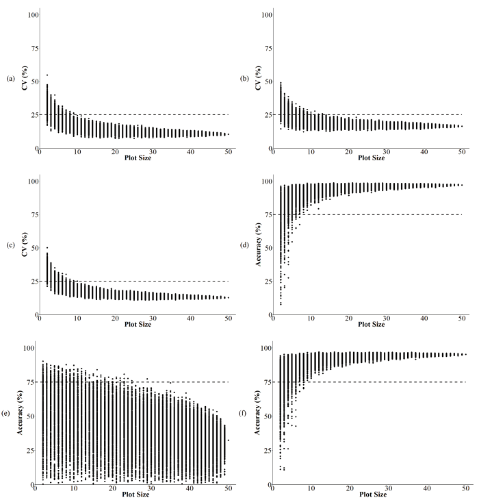
Figure 1
Dispersion of coefficients of variation (CV%) and accuracies (rĝg) estimated by 1,000 simulations as a function of plot size relative to the coffee yield trait. The traced lines parallel to the axis of the abscissas indicate the pre-established values. (a) CV% for Site 1, (b) rĝgfor Site 1, (c) CV% for Site 2, (d) rĝgfor Site 2, (e) CV% for joint analysis, and (f) rĝg for joint analysis.
In classification of the treatments using 50 plants, only two treatments were classified in the first group for Site 2, and five treatments were classified as best by the Scott-Knott grouping test for the joint analysis (Table 2). For Site 1, a significance in the differences between treatments was not detected; therefore, the Scott-Knott test for this Site was not performed. Coincidence in classification of the treatments was greater than 95% for all treatments in the best group, with plot size above 19 plants per plot for Site 2 (Figure 2a). For the joint analysis, a coincidence greater than 95% was obtained with 17 plants per plot (Figure 2b).
| Site 2 | Joint Analysis | |||
| Treatment | Mean* | Treatment | Mean | |
| 8 | 2.140 a | 8 | 4.514 a | |
| 1 | 2.098 a | 1 | 4.341 a | |
| 10 | 1.887 b | 7 | 4.182 a | |
| 6 | 1.846 b | 6 | 4.127 a | |
| 7 | 1.762 b | 10 | 4.126 a | |
| 4 | 1.649 b | 12 | 3.730 b | |
| 5 | 1.625 b | 4 | 3.601 b | |
| 12 | 1.481 c | 5 | 3.546 b | |
| 2 | 1.154 d | 2 | 2.966 c | |
| 3 | 1.108 d | 9 | 2.961 c | |
| 9 | 1.069 d | 3 | 2.840 c | |
| 11 | 1.050 d | 11 | 2.836 c | |
The result obtained by coincidence between treatments was not in agreement with the results obtained by CV and dispersion. Thus, it may be concluded that the study of the percentage of coincidence of the treatments ranking leads to obtaining greater plot sizes. This may be associated with other problems of experimental planning, such as the number of replications or even the small variation among the treatments.
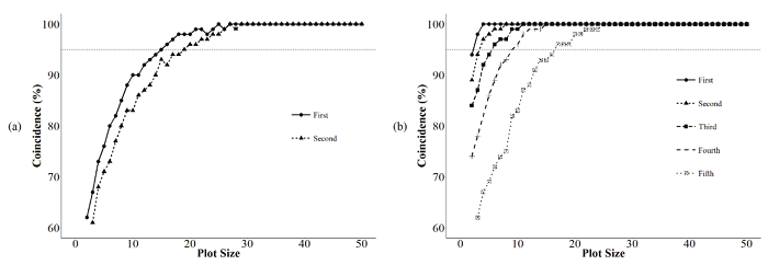
Figure 2
Percentage of coincidence between the classification of the treatments in the best group by Scott-Knott test for each simulated plot size in relation to the maximum size. (a) Site 2 and (b) joint analysis.
To estimate the plot size by the MMCCV, the parameters required by this method were obtained (Table 3). For the joint analysis, the first-order spatial autocorrelation coefficient was considered equal to zero . In the cases when ( = 0 is considered, the estimated plot size will be more conservative, meaning the largest possible (Paranaíba et al., 2009b).
| Parameters | Site 1 | Site 2 | Joint Analysis |
|
| 0.083 | 0.012 | 0.000 |
|
| 3.880 | 1.570 | 3.650 |
|
| 2.480 | 0.510 | 2.710 |
The plot size for Site 1 was the smallest, with 7 plants per plot, followed by Site 2, with 8 plants per plot. The plot size with the information obtained by the joint analysis was the median, with 7.42 plants per plot (Figure 3). Interestingly, even with the genotyping by environment interaction (G x E) detected for the joint analysis, the estimated plot size was equivalent to the analysis for each separate Site. This is because the MMCCV does not incorporate any information about the G x E interaction in its formula. Thus, a plot size that includes all situations in this study is eight plants per plot. According to Paranaíba et al. (2009b) and Lúcio et al. (2012), this method is most adequate for obtaining plot size for crops because it does not need to cluster the basic units to estimate the optimum plot size, making the calculations easier.
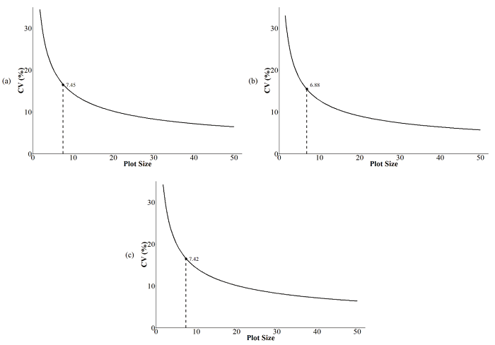
Figure 3
Relationship between coefficient of variation and plot size for the MCCVM. (a) Site 1, (b) Site 2, and (c) joint analysis.
The coefficients of determination of the model were high for the LPSMM for all situations (Site 1, Site 2, and joint analysis), which reveals a good fit of the data to the model and, consequently, good reliability of the estimates of plot size (Table 4).
| Parameters | Site 1 | Site 2 | Joint Analysis |
| β0 | 31.71 | 31.32 | 32.65 |
| β1 | -1.34 | -1.52 | -1.57 |
| CVP | 17.30 | 11.86 | 14.05 |
| X0 | 10.78 | 12.77 | 11.86 |
| R2 (%) | 89.90 | 90.20 | 90.10 |
Similar results were found for radish (Silva, Campos, Morais, Cogo, & Zambon, 2012), maize (Cargnelutti Filho et al., 2011) and black oat (Cargnelutti Filho et al., 2014). As a result of using this model for both Sites and joint analysis, the estimated plot sizes were very similar, varying from 10 to 13 plants per plot (Figure 4).
Different plot sizes were estimated by the MCCVM and LPSMM, agreeing with the plot size found by (Cargnelutti Filho et al., 2011) for maize. For wheat and cassava, these two methods had similar results when Paranaíba et al. (2009b) compared them to estimate the optimum plot sizes in different experiments. These results prove that these different methods can lead to similar estimates of plot size with different crops. Even though there was a difference between the estimates of plot size, the focus of this study was not to evaluate which method of estimation is more precise.
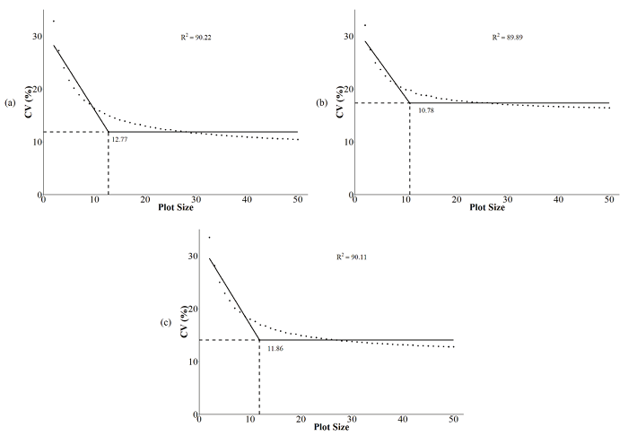
Figure 4
Relationship between the coefficient of variation (CV%) and the plot size for LPSMM. (a) Site 1, (b) Site 2, and (c) joint analysis.
In light of the results found by the different methodologies, it may be inferred that a plot size less than seven plants per plot would not be advisable and that a plot size greater than 19 plants would not bring about additional gains. It was shown in this study that plots smaller than seven plants per plot might not provide trustworthy comparisons between treatments, and they generate a low experimental precision.
The use of larger plots requires a larger experimental area and greater expense, which at times limits the researcher in evaluating a larger number of genotypes. Field experiments with perennial arboreal crops such as coffee usually occupy large areas due to the plant size and the spacing required to manage this crop. Many experiments use large plots with a small number of replicates to reduce the experimental area, manpower, and costs (Rosseti, 2002). However, this can decrease the experimental efficiency, make the application of statistical tests difficult and reduce the ability to detect real differences between treatments.
A benefit of using smaller plots is the ability to increase the number of replicates, allowing better estimations of the experimental error, treatments and parameter effects and a higher accuracy of the statistical tests (Rosseti, 2002). We can recommend smaller plots when it is possible to increase the number of replicates, but we do not advise using plots with fewer than 7 plants.
Conclusion
The number of plants per plot affects the experimental precision when evaluating coffee yield. Experimental plots composed of seven to 19 plants are sufficient for obtaining worthy estimates of parameters of interest for selecting the best cultivars, with high experimental precision.
Acknowledgements
Thanks are due to Conselho Nacional de Desenvolvimento Científico e Tecnológico (CNPq), Fundação de Amparo à Pesquisa do Estado de Minas Gerais (FAPEMIG), Coordenação de Aperfeiçoamento de Pessoal de Nível Superior (CAPES) for the grants and financial support and EPAMIG for providing the experiments
References
Banzatto, D. A., & Kronka, S. N. (2006). Experimentação Agrícola (4a ed.). Jaboticabal, SP: Funep.
Botelho, C. E., Nazareno, A., Mendes, G., Carvalho, G. R., & Ferreira, G. (2007). Seleção de progênies F 4 de cafeeiros obtidas pelo cruzamento de Icatu com Catimor. Revista Ceres, 57(3), 274-281. DOI: 10.1590/S0034-737X2010000300010.
Cargnelutti Filho, A., Alves, B. M., Toebe, M., Burin, C., Santos, G. O., Facco, G., … Stefanello, R. B. (2014). Plot size and number of repetitions in black oat. Ciência Rural, 44(10), 1732-1739. DOI: 10.1590/0103-8478cr20131466
Cargnelutti Filho, A., Toebe, M., Burin, C., Casarotto, G., & Lúcio, A. D. (2011). Métodos de estimativa do tamanho ótimo de parcelas experimentais de híbridos de milho simples , triplo e duplo. Ciência Rural, 41(9), 1509-1516. DOI: 10.1590/S0103-84782011000900004
Cipriano, P. E., Cogo, F. D., Campos, K. A., Almeida, S. L. S., & Morais, A. R. (2012). Suficiência amostral para mudas de cafeeiro cv . Rubi. Revista Agroambiental, 4(1), 61-66. DOI: 10.18406/2316-1817v4n12012375
Dias, K. O. D. G., Gonçalves, F. M. A., Souza Sobrinho, F., Nunes, J. A. R., Teixeira, D. H. L., Moraes, B. F. X., & Benites, F. R. G. (2013). Tamanho de parcela e efeito de bordadura no melhoramento de Urochloa ruziziensis. Pesquisa Agropecuária Brasileira, 48(11), 1426-1431. DOI: 10.1590/S0100-204X2013001100002
Leite, M. S. d. O., Peternelli, L. A., Barbosa, M. H. P., Cecon, P. R., & Cruz, C. D. (2009). Sample size for full-sib family evaluation in sugarcane. Pesquisa Agropecuária Brasileira, 44(12), 1562-1574. DOI: 10.1590/S0100-204X2009001200002
Lorentz, L. H., Erichsen, R., & Lúcio, A. D. (2012). Proposta de método para estimação de tamanho de parcela para culturas agrícolas. Revista Ceres, 59(6), 772-780. DOI: 10.1590/S0034-737X2012000600006
Lúcio, A. D., Haesbaert, F. M., Santos, D., Schwertner, D. V, & Brunes, R. R. (2012). Tamanhos de amostra e de parcela para variáveis de crescimento e produtivas de tomateiro. Horticultura Brasileira, 30(4), 660-668. DOI: 10.1590/S0102-05362012000400016
Morais, A. R., Scalco, M. S., Colombo, A., Faria, M. A., Carvalho, C. H. M., & Paiva, L. C. (2005). Planos de amostragem no desenvolvimento inicial do cafeeiro sob irrigação. Revista Brasileira de Engenharia Agrícola e Ambiental, 9(4), 510-514. DOI: 10.1590/S1415-43662005000400011
Paiva, R. F., Mendes, A. N. G., Carvalho, G. R., Rezende, J. C., Ferreira, A. D., & Carvalho, A. M. (2012). Comportamento de cultivares de cafeeiros C. Arabica L. enxertados sobre cultivar “Apoatã IAC 2258” (Coffea canephora). Ciência Rural, 42(7), 1155-1160. DOI: 10.1590/S0103-84782012000700003.
Paranaíba, P. F., Ferreira, D. F., & Morais, A. R. (2009a). Tamanho ótimo de parcelas experimentais: proposição de metodos de estimação. Revista Brasileira de Biometria, 27(2), 255-268.
Paranaíba, P. F., Morais, A. R., & Ferreira, D. F. (2009b). Tamanho ótimo de parcelas experimentais: Comparação de métodos em experimentos de trigo e mandioca. Revista Brasileira de Biometria, 27(1), 81-90.
Pinto, M. F., Carvalho, G. R., Botelho, C. E., Gonçalves, F. M. A., Rezende, J. C., & Ferreira, A. D. (2012a). Eficiência na seleção de progênies de cafeeiro avaliadas em Minas Gerais. Bragantia, 71(1), 1-7. DOI: 10.1590/S0006-87052012005000008
Pinto, M. F., Carvalho, G. R., Botelho, C. E., Rezende, J. C., Andrade, V. T., Carvalho, J. P. F., & Carvalho, F. (2012b). Seleção de progênies de cafeeiro derivadas de catuaí com icatu e híbrido de timor. Coffee Science, 7(3), 215-222.
R Core Team. (2015). R: A language and environment for statistical computing. Vienna, AU: R Foundation for Statistical Computing.
Ramalho, M. A. P., Ferreira, D. F., & Oliveira, A. C. (2012). Experimentação em genética e melhoramento de plantas (3a ed.). Lavras, MG: UFLA.
Resende, M. D. V., & Duarte, J. B. (2007). Precisão e controle de qualidade em experimentos de avaliação de cultivares. Pesquisa Agropecuária Tropical, 37(3), 182-194.
Rosseti, A. G. (2002). Influência da área da parcela e do número de repetições na precisão de experimentos com arbóreas. Pesquisa Agropecuária Brasileira, 37(4), 433-438. DOI: 10.1590/S0100-204X2002000400002
Scott, A., & Knott, M. (1974). Cluster-analisys method for grouping means in analisys of variance. Biometrics, 30(3), 507-512. DOI: 10.2307/2529204
Silva, L. F. O., Campos, K. A., Morais, A. R., Cogo, F. D., & Zambon, C. R. (2012). Tamanho ótimo de parcela para experimentos com rabanetes. Revista Ceres, 59(5), 624-629. DOI: 10.1590/S0034-737X2012000500007
Steel, R. G. D., Torrie, J. H., & Dickey, D. A. (1997). Principles and procedures of statistics: A biometrical approach (3rd ed.). New York, US: McGraw-Hill Book Company.
Storck, L. (2011). Partial collection of data on potato yield for experimental planning. Field Crops Research, 121(2), 286-290. DOI: 10.1016/j.fcr.2010.12.018
Storck, L., Filho, A. C., Lopes, S. J., Toebe, M., & Silveira, T. R. (2010). Experimental plan for single, double and triple hybrid corn. Maydica, 55(1), 27-32. DOI: 10.1590/S0103-90162007000100005
Storck, L., Lopes, S. J., Lúcio, A. D., & Filho, A. C. (2011). Optimum plot size and number of replications related to selective precision. Ciência Rural, 41(3), 390-396. DOI: 10.1590/S0103-84782011000300005
Author notes
*Author for correspondence. E-mail: avelar@ufla.br