Engenharia Mecânica
Modeling and experimental tests of a copper thermosyphon
Modelagem e testes experimentais de um termossifão de cobre
Modeling and experimental tests of a copper thermosyphon
Acta Scientiarum. Technology, vol. 39, no. 1, pp. 59-68, 2017
Universidade Estadual de Maringá

This work is licensed under Creative Commons Attribution-NonCommercial-NoDerivs 4.0 International.
Received: 27 August 2015
Accepted: 09 November 2015
Abstract: Electrical energy, solar energy, and/or direct combustion of a fuel are the most common thermal sources for home water heating. In recent years, the use of solar energy has become popular because it is a renewable and economic energy source. Among the solar collectors, those assisted by thermosyphons are more efficient; therefore, they can enhance the heat transfer to water. A thermosyphon is basically a sealed tube filled with a working fluid and, normally, it has three regions: the evaporator, the adiabatic section and the condenser. The great advantage of this device is that the thermal resistance to heat transfer between its regions is very small, and as a result, there is a small temperature difference. This article aims to model a thermosyphon by using correlations based on its operation limits. This modeling will be used as a design tool for compact solar collectors assisted by thermosyphons. Based on the results obtained with the mathematical modeling, one copper thermosyphon, with deionized water as the working fluid, was developed and experimentally tested. The tests were carried out for a heat load varying from 30 to 60W in a vertical position. The theoretical and experimental results were compared to verify the mathematical model.
Keywords: solar collector, thermosyphons, operation limit, experiment.
Resumo: Energia elétrica, energia solar e/ou combustão direta de um combustível são as principais fontes térmicas para aquecimento doméstico de água. Nos últimos anos, a utilização de energia solar tornou-se popular porque ela é uma energia renovável e econômica. Dentre os coletores solares, os coletores assistidos por termossifões são os mais eficientes, portanto, eles podem melhorar a transferência de calor para a água. Um termossifão é basicamente um tubo selado preenchido com um fluido de trabalho e, normalmente, possui três regiões: o evaporador, a seção adiabática e o condensador. A grande vantagem deste dispositivo é que a resistência térmica para a transferência de calor entre suas regiões é muito pequena e, como resultado, existe uma pequena diferença de temperatura. Este artigo tem como objetivo modelar um termossifão utilizando correlações baseadas em seus limites de operação. Esta modelagem será utilizada como uma ferramenta de projeto para coletores solares compactos assistidos por termossifões. Baseado nos resultados obtidos com o modelo matemático, um termossifão de cobre, com água deionizada como fluido de trabalho, foi desenvolvido e testado experimentalmente. Os testes foram realizados para uma potência variando de 30 a 60W em uma posição vertical. Os resultados teóricos e experimentais foram comparados para verificar o modelo matemático.
Palavras-chave: coletor solar, termossifões, limite de operação, experimental.
Introduction
Water heating systems for domestic use in Brazil can have an energy source of electrical energy, solar energy, and/or direct burning of a particular fuel (LPG or natural gas) in a gas burner. Due to the water crisis that the country is facing, the high cost of heating water by electricity is increasingly being replaced by heating through fuel combustion in a gas burner or by the use of a solar collector; and in some cases, both technologies are used together.
The most common solar collector used in Brazil is the flat plate. This type of solar collector is a Brazilian technology; however, they occupy large areas on building roof tops. A more thermally efficient solar collector is the evacuated tube solar collector (thermosyphon solar collector). This type of solar collector is more efficient because it uses thermosyphons in order to enhance the transfer of heat for water heating. However, there are few applications of thermosyphon solar collectors in Brazil and Brazilian companies do not have the manufacturing technology.
Several researchers have studied the application of heat pipes and thermosyphons in solar collectors for heating water in the interest of domestic use with different configurations (Hussein, Mohamad, & El-Asfouri, 1999a, 1999b; Ismail & Abogderah, 1998; Oliveti & Arcuri, 1996).
The solar collectors tested by Oliveti and Arcuri (1996) and Hussein et al. (1999a, 1999b) were assisted by thermosyphons with water as the working fluid. On the other hand, Ismail and Abogderah (1998) used heat pipes with methanol as the working fluid in the solar collectors. Abreu and Colle (2004) presented a different configuration of the settings above. While the other researchers used straight tube thermosyphons, Abreu and Colle (2004) developed a condenser with curved geometry to allow a better coupling between the condenser region and the heat sink.
Azad (2008) accomplished a theoretical and experimental study on the thermal performance of thermosyphon solar collectors. He worked on a copper collector with six thermosyphons with an external diameter of 12.7 mm and a length of 1,850 mm. The tests were performed outdoor in Tehran (Iran) and the thermal efficiency was based on ASHRAE 93-1986 method.
Chien et al. (2011) also made a theoretical and experimental study regarding a solar collector assisted by thermosyphons. They used the method of equivalent thermal resistances for the theoretical study, and for the experiment, they tested the solar collectors under different inclination angles and heat loads.
Azad (2012) manufactured three heat pipe solar collectors with tubes of different shapes and with a total length ranging from 1.55 to 1.90 m. All heat pipes used a stainless steel wire mesh of 100 and ethanol as the working fluid. The solar collectors were tested outdoor in Tehran (Iran).
Du, Hu, and Kolhe (2013) manufactured a solar collector assisted by twenty heat pipes and tested it outdoors in Nanjing (China). Each heat pipe had an evaporator outer diameter of 8 mm and length of 1,660 mm, and a condenser outer diameter of 14 mm and length of 83 mm. The heat pipes were inserted into a borosilicate glass tube with a diameter of 70 mm and a length of 1,730 mm. In the annular space between the glass tube and an evacuation process, up to 0.05 Pa was accomplished (absolute pressure).
Deng et al. (2013) constructed and tested a solar collector assisted by an array of micro heat pipes made of aluminum. The heat pipes used acetone as the working fluid and the capillary structure was composed by grooves with hydraulic diameter varying between 0.4 and 1.0 mm.
According to this review, the development process of thermosyphons and heat pipes for solar collectors is not presented. In other words, for this specific application, the manufacturing process as well as the necessary experimental tests for qualifying these kinds of devices are not shown. Thus, this paper aims to present the steps to develop thermosyphons for application in solar collectors.
Material and methods
Operation limit model for thermosyphons
The mathematical model presented here consists of determining the operational limits for thermosyphons. These limits are entrainment, sonic, viscous, drying, and boiling. For each one of them, specific correlations will be used for their evaluations.
One thermosyphon is schematically represented in Figure 1, which is composed of three regions: the evaporator section (where the heat load is supplied), the adiabatic section, and the condenser section (where the heat is removed). The thermosyphon works in the following way: first, heat is supplied in the evaporator section causing the vaporization of the inner working fluid; second, due to the pressure difference, the generated vapour flows to the thermosyphon cooled region (condenser section) where heat is rejected by the cold source (water or air flow passing outside the tubes) and the vapour condenses inside; third, the condensate fluid returns to the evaporator by gravity, completing the cycle.
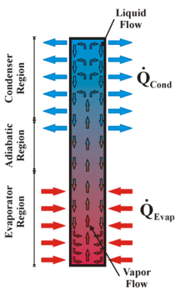
Figure 1
Schematic representation of a typical thermosyphon.
Since the thermosyphon is assisted by gravity, the condenser region must be located above the evaporator region at a minimal tilt angle. The adiabatic region is located between the evaporator and the condenser (it has variable size or may not exist in some cases).
Operation limit model
The limit model was implemented and simulated using the software EESTM (Engineering Equation SolverTM).
Entrainment limit
As the heat load applied to the evaporator is increased, the vapor velocity increases and may reach a higher velocity than the liquid velocity. That is, the shear forces on the liquid-vapor interface can be significant. Thus, if the shear forces are greater than the forces caused by the liquid surface tension, droplets can be dragged from the liquid. As a consequence, the entrainment limit can be reached.
The entrainment limit estimates the maximum value of heat transfer rate that leads this effect to take place within the thermosyphon. The main cause for this limit to be reached is the excess of working fluid in the condenser or the lack of working fluid in the evaporator.
According to Groll and Rosler (1992) and Mantelli (2013), some expressions have been developed for the entrainment limit estimation. The correlation shown in Equation (1) has been proposed to determine the maximum heat transfer for the entrainment limit.
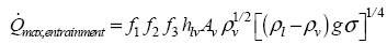 (1)
(1)where,
f1, f2, and f3 are parameters listed as follow; hlv is the vaporization latent heat; ρv is the vapor density; ρl is the liquid density; g is the gravitational acceleration; is the surface tension; and Av is the vapor core area.
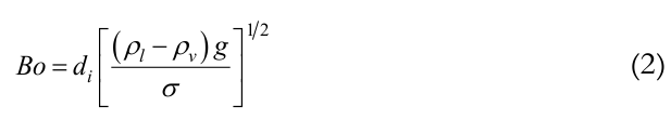
The parameter f1 is the Bond number (Bo), Equation (2), defined as the ratio between gravity and surface tension forces,
 (2)
(2)where,
di is the tube inner diameter.
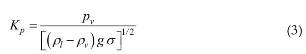
The parameter f2 is a function of the dimensionless parameter Kp, given by Equation (3):
 (3)
(3)where,
pv is the vapor pressure.
For Kp ≤ 4.104, f2 = Kp– 0.17 and for Kp > 4.104, f2 = 0.165.
The parameter f3 is a factor which corrects the Eq. (1) for the thermosyphon inclination and it is also a function of the Bond number. According to Mantelli (2013) for vertical position, f3 = 1.
Sonic limit
The sonic limit represents the heat applied to the thermosyphon when vapor reaches sonic velocity. It can be more commonly achieved by thermosyphons using liquid metal as the working fluid and it is influenced by the size of the vapor core. Sonic limits can be reached during the start-up and at steady state conditions. If this limit is reached, the vapor usually located in the core of the thermosyphon is blocked by a shock wave. This phenomenon causes a temperature increase in this region and can be expressed by Equation (4) which was proposed by Busse (1973):
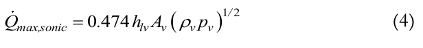 (4)
(4)Viscous limit
In situations in which the thermosyphon works at low temperature levels, the pressure gradient between the evaporator and the condenser is very small. When the forces caused by such low pressure gradient are lower than the viscous forces, vapor flow does not take place in the thermosyphon. This characterizes the viscous limit. Busse (1973) proposed a correlation, Equation (5), for this limit:
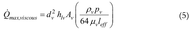 (5)
(5)where,
dv is the vapor core diameter, μv is the vapor dynamic viscosity, and leff is the effective length given by
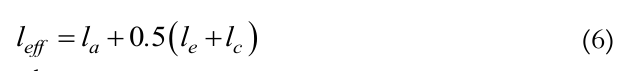 (6)
(6)where,
la is the adiabatic section length, le is the evaporator region length, and lc is the condenser region length.
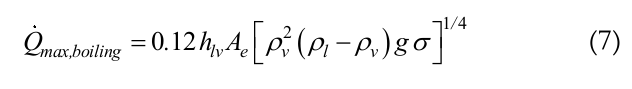
Boiling limit
The boiling limit occurs when there is a large amount of working fluid in the thermosyphon and the evaporator region is heated with high heat fluxes. It occurs at the transition between the boiling processes of pool boiling and evaporation in film, when the heat flux is critical. As a result, bubbles are formed and adhered to this film, causing insulation of the inner pipe wall. Since the vapor thermal conductivity is low, the wall temperature increases and it may reach, in extreme cases, the melting point of the metal material. An expression is proposed in Peterson (1994), Equation (7), to estimate the maximum heat transfer rate for the boiling limit:
 (7)
(7)where,
Ae is the evaporator area.
Heat Transfer Analysis
This section presents the heat transfer analysis based on the correlations using the experimental data as input.
Calculation of the heat transferred to the thermosyphon
In order to calculate the heat transfer rate that is transferred to the thermosyphon, a control volume is established according to Figure 2.
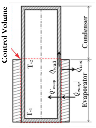
Figure 2.
Energy balance in evaporator section.
Applying an energy balance in the control volume of Figure 2, the Equation (8) can be obtained:
 (8)
(8)where,
 is the heat transfer rate supplied to the evaporator by the heat system (skin heater/electric resistor), Equation (9);
  is the heat transfer rate lost axially through the tube wall, Equation (10); and
  is the heat transfer rate lost through the insulation, Equation (11).
 (9)
(9)
 (10)
(10)
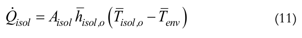 (11)
(11)where,
I is the electric current, V is the voltage, is the copper thermal conductivity, Aw is the wall cross area,  is the outer evaporator average temperature,
  is the outer condenser average temperature, Aisol is the insulation area,
  is the outer insulation average heat transfer coefficient,
  is the outer insulation average temperature, and
  is the environment average temperature.
According to Bergman, Lavine, Incropera and DeWitt (2012) the heat transfer coefficient by natural convection at outer insulation can be estimated by the Equations (12) and (13), Churchill and Chu’s correlation. That is,
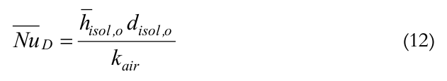 (12)
(12)
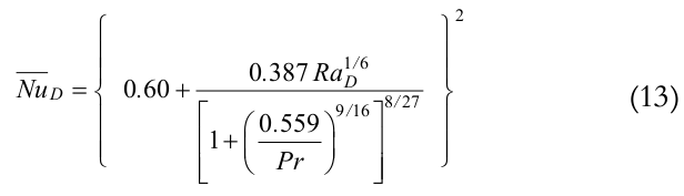 (13)
(13)where,
 is the average Nusselt number, disol,o is the outer insulation diameter, Kair is the air thermal conductivity,
 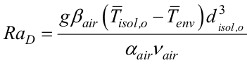 is the Rayleigh number, and Pr is the Prandtl number.
Mass transfer rate of internal flow
The calculation of the thermosyphon’s internal mass transfer rate, mi, can be estimated by Equation (14), neglecting the sensible heat variation along the evaporator region.
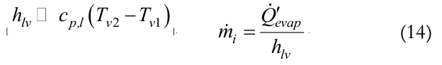 (14)
(14)Heat transfer coefficient calculation for the internal region of the condenser
To determine the internal heat transfer coefficient for the condenser region, the operation temperature must be primarily estimated. Thus, an equivalent thermal circuit presented in Figure 3 is proposed for determining the operation temperature Top.
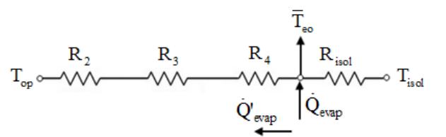
Figure 3.
Equivalent thermal circuit.
where,
Top is the operating temperature, is the outer evaporator average temperature, Tisol is the outer insulation average temperature, R2 is the thermal resistance associated to the wall conduction, Equation (15), R3 is the thermal resistance associated to the inner evaporation, Equation (16), R3p is for pool boiling using Equation (17) and R3fis for evaporation in film using Equation (18), and R4is the thermal resistance associated with the liquid-vapor interface, Equation (19),
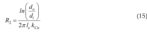 (15)
(15)
 (16)
(16)
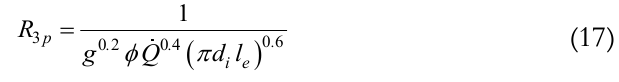 (17)
(17)
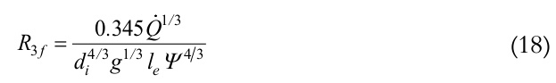 (18)
(18)
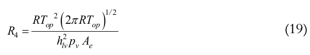 (19)
(19)where,
do is outer diameter, F is filling ratio (defined as the ratio between the volume of working fluid and volume of the evaporator), R is the universal gas constant, ϕ and Ψ are given by
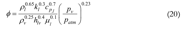 (20)
(20)
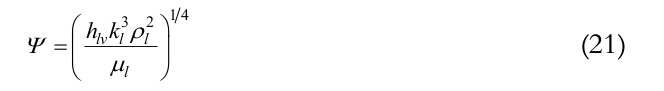 (21)
(21)where,
kl is the liquid thermal conductivity, cp,lis the liquid specific heat at constant pressure, and μlis the liquid dynamic viscosity.
Therefore, based on the analysis of the equivalent thermal circuit, the Eq. (22) can be determined as:
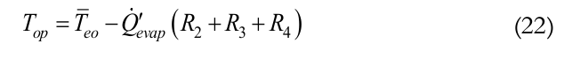 (22)
(22)In order to estimate the internal heat transfer coefficient into the condenser area, the condensate thermal resistance, Rcond, can be used. This thermal resistance is given by Equation (23).
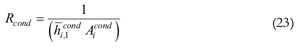 (23)
(23)Based on the Nusselt analysis for condensation, Groll and Rosler (1992) suggest a correlation for the condensation thermal resistance:
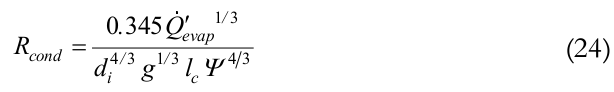 (24)
(24)where
 is the condenser internal average heat transfer coefficient, obtained by Groll and Rosler correlation, and Aicondis the condenser inner area. On the other hand, Mantelli (2013) state that the inner average heat transfer coefficient in the condenser can be estimated through the correlation obtained by Kaminaga, Equations (25) to (27):
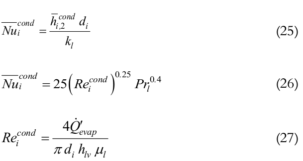 (25-27)
where,
 is the condenser inner average Nusselt number,
  is condenser inner average heat transfer coefficient obtained by the Kaminaga correlation, Reicond is the condenser inner Reynolds number and Prl is the liquid Prandtl number.
Experiment
The methodology to manufacture the thermosyphon was based on Santos, Krambeck, Santos, and Antonini (2014). The thermosyphon was produced by copper tube with an outer diameter of 12.7 mm, a wall thickness of 1 mm, and a total length of 500 mm (Figure 4). The lengths of the evaporator and condenser are 150 and 350 mm, respectively. There is no adiabatic region. The thermosyphon was filled with 45.38 ml of deionized water.
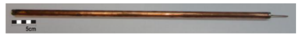
Figure 4.
Thermosyphon made of cooper.
Figure 5 shows the test rig which is composed by a copper thermosyphon, a power supply (AgilentTM U8002A), a data acquisition system (AgilentTM 34970A with 20 channels), a computer (Intel CoreTM i5 3.30Ghz), an airflow fan (WMRTM P/N2123XST) and a digital anemometer (MinipaTM MDA-20).
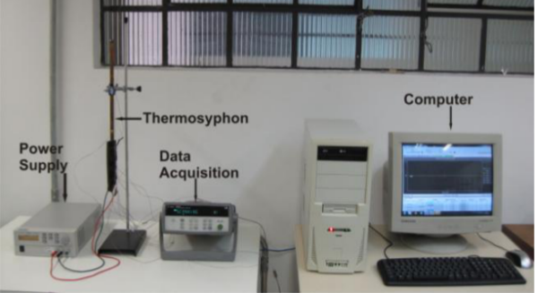
Figure 5.
Test rig for the tests of copper thermosyphon cooled by air forced convection.
The evaporator of the thermosyphon was heated using a wire electric resistor (evaporator region at Figure 6) and the condenser was cooled by air forced convection. The heat load applied to the evaporator varied from 30 to 60 W.
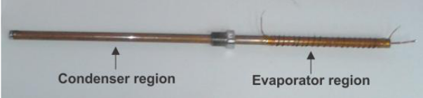
Figure 6.
Condenser and evaporator regions.
The thermosyphon was tested at vertical position and a digital anemometer was used to measure the air velocity (approximately 5.6 ms-1). The temperatures along the thermosyphon’s outer surface were measured using 11 thermocouples (T-type): 4 thermocouples at the evaporator (Tevap1, Tevap2, Tevap3, and Tevap4), 4 thermocouples at the condenser (Tcond1, Tcond2, Tcond3, and Tcond4) and 3 thermocouples at the thermal insulation (Tisol1, Tisol2, and Tisol3), as shown in Figure 7.
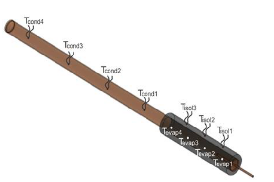
Figure 7.
Thermocouples positions on the outer surface of thermosyphon and insulation.
The experimental uncertainties were estimated using the ISO-GUM method and taking into account the data acquisition and power supply uncertainties. Thus, the temperature uncertainty was estimated as ± 0.8oC and the uncertainty of the heat load applied to the evaporator was ± 0.53W.
Results and discussion
The experimental and theoretical results concerning the analysis of the thermosyphon are presented in this section.
Operation limits analysis
According to the mathematical model, for the operation temperature variation from 30 up to 110oC, the operation limits varied as shown in Figure 8. Figure 8(a) presents the entrainment, viscous, and sonic limits and, the boiling limit is shown in Figure 8(b).
Results showed that, as the temperature increases, all limits increase and the entrainment limit is the less restrictive limit until 85oC. After this temperature, the viscous limit exceeds the entrainment limit, becoming the less restrictive limit. On the other hand, the ranges of sonic, viscous, and boiling limits are close together for the temperature variation from 30 to 45oC. In this temperature range, the boiling limit varied from 1,568 to 2,246 W; the viscous limit varied from 2,266 to 10,399 W; and the sonic limit varied from 2,486 to 5,404 W. Thus, as a result, the boiling limit was the most restrictive.
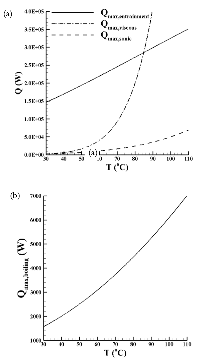
Figure 8.
Analsys of operation limits: (a) entrainment, viscous, and sonic limits and (b) boiling limit.
Temperature along the thermosyphon as a function of heat load
The experimental results as a function of the heat load applied in the evaporator region are presented in Figure 9.
First, a heat load of 30W was applied to the evaporator of the thermosyphon and it is noticed that all temperatures along the external surface of the thermosyphon (Tevap1, Tevap2, Tevap3, Tevap4, Tcond1, Tcond2, Tcond3, and Tcond4) increase rapidly. After approximately 100 s, the thermal behaviour of these temperatures tends to the steady state regime. Thus, it can be stated that it had a successful start-up. The steady state was reached at approximately 200 s.
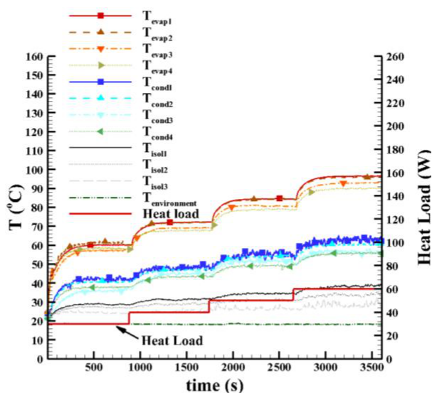
Figure 9.
Temperature along the thermosyphon as a function of power and time applied.
After 15 min. (900 s), the heat load was increased to 40 W and a similar thermal behaviour of the thermosyphon temperatures was observed. The heat load varied from 40 to 50W and, finally, from 50 to 60W. Note that for all heat loads applied, the thermosyphon reached the steady state condition. The maximum temperature measured was 97oC in the evaporator region for the heat load of 60W. The maximum temperature measured in the condenser was 61°C and in the insulation was 39oC, both for 60W.
Heat transfer analysis
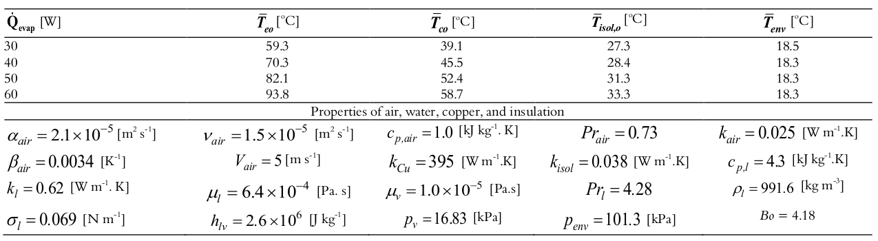
Table 1 shows the main experimental data and properties used for the heat transfer analysis presented in the present work.
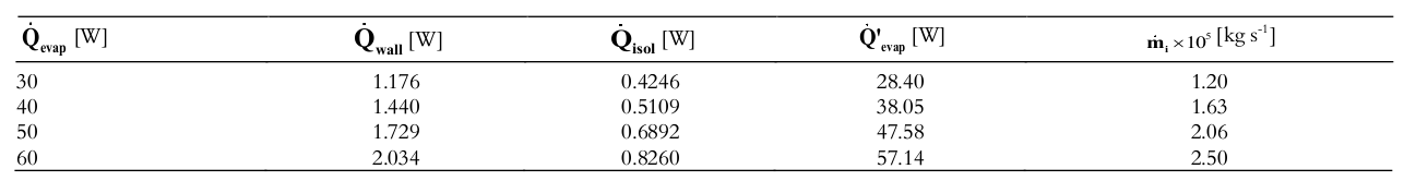
Table 2 lists the results of the heat transfer analysis as a function of the heat transfer rates: applied to the evaporator region, lost through the insulation and the thermosyphon wall, transferred into the thermosyphon, and internal mass flow rate.
It is observed that when a heat load of 30 W was applied, 3.9 % of the heat was transferred through the tube wall, 1.4% was transferred through the insulation, and 94.7% was transferred into the evaporator of the thermosyphon. The estimated percentages for the other heat loads (40, 50, and 60W) are very similar to these. Regarding the internal mass flow rate, the variation is very small (order of 10–5 kg s–1).
Analysis of the internal heat transfer coefficient in the condenser region
Table 3 presents the values of the internal heat transfer coefficients into the condenser region as a function of the heat load.
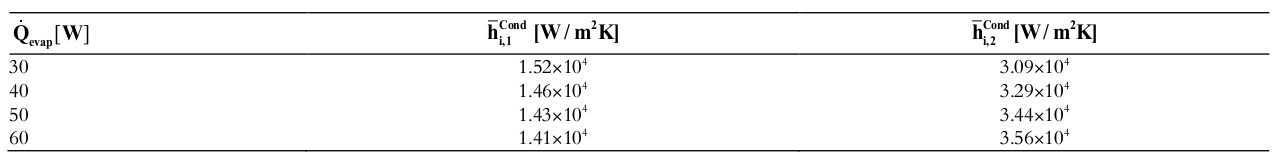
From the two correlations presented before and the experimental data obtained through the heat transfer analysis, it is possible to estimate the coefficients in this section. is calculated using Groll and Rosler correlation, Equation (24), and using Kaminaga correlation, Equation (26). Note that is 10 times greater than . Thus, the value of is more conservative. However, the development of a more sophisticated experiment is necessary in order to measure the inner heat transfer coefficient of the condenser region.
Comparison between theoretical and experimental results
Figure 8 shows the theoretical results of the operation limits as a function of operation temperature variation (30 up to 110oC). Here, the real operation temperature was estimated, using Eq. (22), regarding the heat load applied to the evaporator.
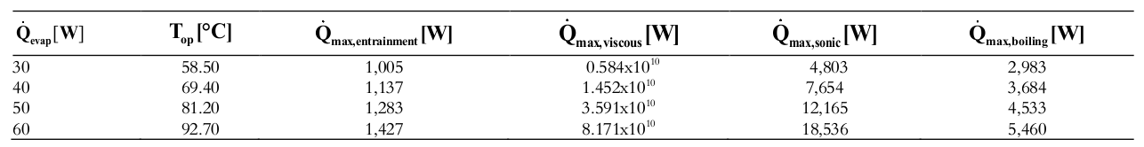
Table 4 presents the maximum heat transfer rates for each operating limit taking into account the real operating temperature.
From Table 4, it is possible to observe that the heat transfer rate obtained for the viscous limit is much higher than the other limits for the all heat loads. It is also observed that for all heat loads applied to the evaporator, the maximum heat transfer rates obtained for the entrainment limit are the lowest one, varying from 1,005 to 1,427W. Therefore, it can be stated that the proposed thermosyphon could operate under higher heat loads than the ones applied. However, for security reasons, the accomplishment of these tests was possible due to the temperature limitation imposed (maximum temperature of 120oC).
Conclusion
This paper presented a theoretical and experimental analysis of a copper thermosyphon with deionized water as the working fluid. The device was cooled by air forced convection. Regarding the theoretical analysis, the entrainment, viscous, sonic, and boiling limits were evaluated for a temperature ranging from 30 to 110oC. It was observed in the analysis that the maximum heat transfer rates obtained were very high when compared to the heat load applied to the evaporator in the experiment. It was also noticed that the heat transfer rates obtained for the boiling limit were the less restrictive ones.
Regarding the experimental analysis, the thermosyphon was tested at vertical position under heat loads of 30, 40, 50, and 60W. The device worked satisfactorily obtaining successful start-up, and reaching steady state condition for all heat loads. The thermosyphon took about 200 s to reach the steady state for heat load of 30W, and the maximum temperature of 97oC was measured at the evaporator region for 60W.
A heat transfer analysis was performed using the experimental data obtained from the tests, in which it was estimated the operating temperature inside the evaporator region (92.7oC for 60W, for instance). The operating temperatures obtained in the experiments were used to determine the operating limits. For all the heat loads, the heat transfer rates were estimated for operating limits. The entrainment limit was the lowest one, ranging from 1,005 to 1,427W. Therefore, it is possible to attest that the thermosyphon developed here could operate under much higher heat loads without reaching any operating limit. However, for safety reasons, it was not possible to perform such tests due to the experimental temperature limitation (120oC). The internal mass flow rate was estimated as an order of 10-5 kg s-1.
Using specific correlations for thermosyphon condensers, together with the mass flow rate calculated from the experimental results, it was possible to determine the internal heat transfer coefficient into the condenser region. The values estimated were in the order of 104 W m-2K ( ) and, when using the second method, the values were in the order of 103 W m-2K ( ).
Therefore, it can be concluded that the methodology used in the development, test, and analysis of the copper thermosyphon presented in this paper proved to be feasible.
References
Abreu, S. L. & Colle S. (2004). An experimental study of two-phase closed thermosyphons for compact solar domestic hot-water systems. Solar Energy, 76(1), 141-145.
Azad, E. (2008). Theoretical and experimental investigation of heat pipe solar collector. Experimental Thermal and Fluid Science, 32(8), 1666-1672.
Azad, E. (2012). Assessment of three types of heat pipe solar collectors. Renewable and Sustainable Energy Reviews, 16(5), 2833-2838.
Bergman, T. L., Lavine, A. S., Incropera, F. P. & DeWitt, D. P. (2012). Fundamentals of heat and mass transfer (6th ed.). New Jersey, US: John Wiley & Sons.
Busse, C. A. (1973). Theory of the ultimate heat transfer limit on cylindrical heat pipes. International Journal of Heat and Mass Transfer, 16(1), 169-186.
Chien, C. C., Kung, C. K., Chang, C. C., Lee, W. S., Jwo, C. S. & Chen, S. L. (2011). Theoretical and experimental investigations of a two-phase thermosyphon solar water heater. Energy, 36(1), 415-423.
Deng, Y., Zhao, Y., Wang, W., Quan, Z., Wang, L. & Yu, D. (2013). Experimental investigation of performance for the novel flat plate solar collector with micro-channel heat pipe array (MHPA-FPC). Applied Thermal Engineering, 54(2), 440-449.
Du, B., Hu, E. & Kolhe, M. (2013). An experimental platform for heat pipe solar collector testing. Renewable and Sustainable Energy Reviews, 17, 119-125.
Groll, M. & Rosler, S. (1992). Operation principles and performance of heat pipes and closed two-phase thermosyphons. Journal of Non-Equilibrium Thermodynamics, 17(2), 91-151.
Hussein, H. M. S., Mohamad, M. A. & El-Asfouri, A. S. (1999a). Optimization of a wickless heat pipe flat solar collector. Energy Conversion and Management, 40(18), 1949-1961.
Hussein, H. M. S., Mohamad, M. A. & El-Asfouri, A. S. (1999b). Transient investigation of a thermosyphon at-plate solar collector. Applied Thermal Engineering, 19(7), 789-800.
Ismail, K. A. R. & Abogderah M. M. (1998). Performance of a heat pipe solar collector. Journal of Solar Energy Engineering, 120(1), 51-59.
Mantelli, M. H. B. (2013). Thermosyphon technology for industrial applications. In L. L. Vasiliev, & S. Kakaç, (Eds.), Heat pipes and solid sorption transformations: fundamentals and practical applications (p. 411-464, Chapter 11). New York, UA: CRC Press.
Oliveti, G. & Arcuri N. (1996). Solar radiation utilisability method in heat pipe panels. Solar Energy, 57(5), 345-360. doi:10.1016/S0038-092X(96)00109-0
Peterson, G. P. (1994). Heat pipes: modeling, testing, and applications. Toronto, CA: John Wiley & Sons.
Santos, P. H. D., Krambeck, L., Santos, D. L. F. & Alves, T, A. (2014). Analysis of a stainless steel heat pipe based on operation limits. International Review of Mechanical Engineering, 8(3), 599-608.
Author notes
thiagoaalves@utfpr.edu.br