Engenharia Mecânica
Influence of damping ratio on a structural optimization design considering a dynamic analysis within the time domain
Influência da taxa de amortecimento no projeto de otimização estrutural considerando análise dinâmica no domínio do tempo
Influence of damping ratio on a structural optimization design considering a dynamic analysis within the time domain
Acta Scientiarum. Technology, vol. 40, 2018
Universidade Estadual de Maringá

This work is licensed under Creative Commons Attribution 4.0 International.
Received: 15 January 2016
Accepted: 23 February 2016
Abstract: Structural optimization has received increasing attention in several different areas of engineering and has been identified as the most challenging and economically rewarding task in the field of structural design. In this context, the current paper proposes a methodology based on Evolutionary Structural Optimization (ESO) that corresponds to an evolutionary procedure applied for topological optimization in which the finite elements with the lowest stress levels are progressively removed from a structure. The optimization studies are applied for structures subjected to a transient dynamic response where different damping ratios are applied in the physical models, since its determination is extremely hard and can even change the structural stiffness in case of elastoplastic regime. Thus, a nonlinear behavior is considered to evaluate the effects for each damping ratio, and elastoplasticity theory for small strains is extended for a von Mises material with linear, isotropic work-hardening. For this purpose it is possible to evaluate a combination of different optimal topologies for the different damping ratios through an algorithm developed in the Python programming language. The stress levels present such a difference for each linear and nonlinear response, which characterizes a marked change in the structural stiffness of each analyzed model.
Keywords: evolutionary structural optimization, dynamic response, damping, finite element method.
Resumo: A otimização estrutural vem recebendo cada vez mais atenção em diversas áreas da engenharia e tem sido identificada como um dos maiores desafios em projeto estrutural. Neste contexto, o presente trabalho propõe uma metodologia baseada na Otimização Estrutural Evolucionária (ESO) que corresponde a um procedimento evolutivo aplicado em otimização topológica em que os elementos finitos com os mais baixos níveis de tensão são progressivamente removidos da estrutura. Os estudos de otimização são aplicados em estruturas sujeitas a uma resposta dinâmica transitória, e diferentes taxas de amortecimento são aplicadas nos modelos físicos, pois a sua determinação é extremamente difícil, podendo inclusive, alterar a rigidez da estrutura em casos de regime elastoplástico. Assim, o comportamento não linear é considerado a fim de se avaliar os seus efeitos para cada taxa de amortecimento, e a teoria da elastoplasticidade para pequenas deformações é estendida a um material de von Mises com encruamento isotrópico linear. Com este propósito é possível avaliar uma combinação das topologias ótimas distintas para as diferentes taxas de amortecimento através de um algoritmo desenvolvido em linguagem de programação Python. Os níveis de tensões apresentaram diferenças significativas para respostas linear e não linear, caracterizando acentuada alteração na rigidez estrutural dos modelos analisados.
Palavras-chave: otimização estrutural evolucionária, resposta dinâmica, amortecimento, método dos elementos finitos.
Introduction
Topology optimization has an extremely important role in several different engineering problems, where the main objective is to establish a final optimal topology within the project domain in relation to the given objective function subject to certain restrictions (Bendsøe & Sigmund, 2003).
In this context, owing to the computational progress, various topology optimization methods have been studied, among which the Evolutionary Structural Optimization (ESO) method stands out. This evolutionary procedure is based on a gradual removal of materials considered inefficient within the project region, which must be discretized using a suitable polynomial approximation in a chosen finite element mesh, where the maximum von Mises stress will be used as an element removal parameter through a rejection criterion (Xie & Steven, 1993).
This technique has already generated several different studies involving static actions in the linear regime, such as those by Huang and Xie (2010) and Xie and Steven (1997). However, little progress has been made under other application conditions. Currently, one of the most interesting optimization problems is associated with the physical properties of an optimized structure. The structural stiffness is dependent on the damping ratio, particularly for higher frequencies. A methodology applied to a dynamic analysis of the structures within the elastoplastic regime, together with the geometric nonlinearity, should therefore be considered to obtain a more reliable structural optimization design.
The basic idea of the ESO methodology is to analyze the complete area where a structure may exist, i.e., the design domain, and based on the chosen objective function, evaluate the effectiveness of each element within the structure, gradually removing the less efficient elements.
For each optimization problem, one or more types of material removal criteria exist, including the stiffness, displacement, pressure, stress level, natural frequency, and critical buckling load.
Material and methods
The optimization of a structure based on its stress level is a process used in many areas of structural mechanics. Through an analysis using the Finite Element Method (FEM), it is possible to determine the level of the structure, which can then be used as an indicator of the efficiency of each element within the structure. The rejection criteria can then be established based on the maximum stress level, in which a material under low stress is considered underutilized and can be removed from the structure (Xie & Steven, 1997). Considering a structure discretized using a proper finite element mesh, the material removal is conveniently represented by excluding the elements from the mesh according to the design criterion adopted.
The stress level at each point can be measured as the overall average of the stress components. For this purpose, the equivalent von Mises stress has been more commonly used for isotropic materials (Xie & Steven, 1997; Tanskanen, 2002; Fernandes et al., 2017).
Thus, after finishing the structural analysis through an FEM, the stress level applied for each element is determined by comparing the equivalent von Mises stress of the element with the maximum equivalent von Mises stress throughout the structure in such a way that all elements that satisfy the condition represented through Equation 1 are excluded from the model.
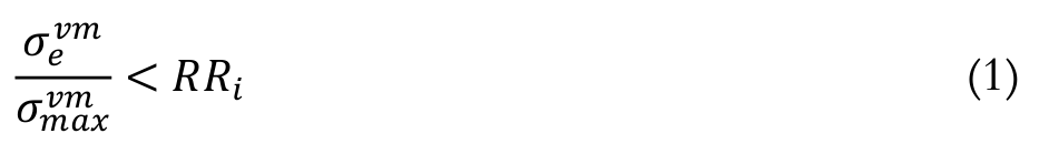 (1)
(1)where:
 is the rejection ratio (
 ) at iteration i,
 is the equivalent von Mises stress of the element, and
 is the maximum equivalent von Mises stress throughout the structure.
The
analysis cycle by FEM with the respective element removal occurs using the same
value until a steady state is reached, i.e., when there are no more elements to
be removed by the current element (Xie & Steven,
1997). This implies that the number of elements removed for each analysis is
not necessarily the same for all iterations. Reaching this state of
equilibrium, but not reaching a stopping criterion of the iterative process (with
the optimum configuration based on the ESO method), the evolutionary process is
reset by adding an evolution ratio ( ). Thus, a new development cycle begins and
is repeated until there are no more elements to be eliminated using this new
rejection ratio. In this way, when a steady state is reached, the
). Thus, a new development cycle begins and
is repeated until there are no more elements to be eliminated using this new
rejection ratio. In this way, when a steady state is reached, the  is
added tor
is
added tor  , as shown in Equation 2:
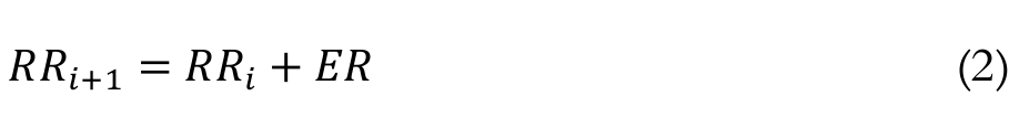 (2)
(2)where:
 is the
  at iteration i + 1, and
 is the evolution ratio.
The initial rejection ratio is generally conditioned to the prescribed values within the range of  . However, there are cases in which, depending on the type of analysis and the discretization of the finite element mesh, it may be necessary to use values higher than 1% owing to the non-removal of the elements. The initial value of RRi is defined empirically according to the user experience for each type of problem. Two evolutionary process stopping criteria can be established, namely, the prescribed final volume (
 and the final rejection ratio (
 ).
).
The main advantages of the ESO methodology are the possibility of monitoring the component shape at every stage of the optimization process, the simplicity of the implementation and execution, the potential application of various types of analysis, and easy integration with any type of commercial software, which provide an excellent alternative of use.
The ESO method creates cavities in a structure from the removal of inefficient elements, regardless of their location in the field, which can result in a numerical instability of the chessboard.
To mitigate the chessboard irregularities, a Nibbling ESO technique has been used, which is an adaptation of the ESO method containing optimization features to control the cavities. This technique evaluates the stress field and checks the possibility of opening cavities within the project domain, resulting in the elimination of only those elements that are present in the contours of the structure, avoiding excessive and unnecessary voids in the optimization process (Lanes & Greco, 2013). The need to create a new cavity within the domain is verified at each iteration, and if necessary, the ESO method is applied. Otherwise, the Nibbling ESO method proceeds with the removal of only elements that are present in the contours of the structure, modifying their shape and size until a new cavity opening is needed.
Regarding the mesh dependency problem, an approach by Kim et al. (2002) has been used, which considers the use of the mean stress of the finite element as the removing criterion in the analysis of the stress levels. When the maximum stress is used, the results become very dependent on the mesh owing to the singularities occurring near the boundary conditions.
For an optimization of linear problems, the ESO method based on the Python programming language using Abaqus® scripting was first implemented by Lanes and Greco (2013). To consider the combined optimization for different damping ratios, a new script was developed.
Physically nonlinear behavior (elastoplastic constitutive model)
The elastoplastic behavior is characterized through a response of the material, which is initially elastic, and from a certain stress level based on an essentially plastic behavior.
The nonlinear behavior of the material is described through
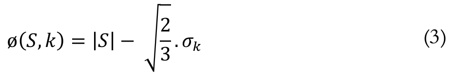
a von Mises criterion suitable for metallic materials with ductility. In this
criterion, the yield function  includes the deviatory stress tensor
  and yield stress with isotropic hardening (
 ), which is described as a
function of the internal variable
), which is described as a
function of the internal variable  , which is related to plastic
deformation (Maute, Schwarz, & Ramm, 1998). To
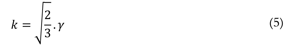
better describe this criterion, Equations 3through 5 can be used.
, which is related to plastic
deformation (Maute, Schwarz, & Ramm, 1998). To
better describe this criterion, Equations 3through 5 can be used.
 (3)
(3)
 (4)
(4)
 (5)
(5)where:
 is the yield function,
 is the deviatory stress tensor,
 is the yield stress with isotropic hardening,
 is the yield stress,
 is the plastic hardening modulus,
 is the internal variable, and
 is the plastic multiplier.
Assuming the presence of small deformations, it can be divided into incremental portions of plastic and elastic deformation. Thus, the additive decomposition rule can be applied according to Equations 6through 9:
 (6)
(6)
 (7)
(7)
 (8)
(8)
 (9)
(9)where:
 is the total deformation increment,
 and
and  correspond to the increments of elastic and
  plastic deformations, respectively, and denotes the elastic tensor of the material
The gradient  is evaluated after each iteration step considering an implicit Euler algorithm. For a plastic deformation to occur, the yield function must be zero, i.e.,
  . If
. If  , only the elastic regime exists, and thus
  . However, when
  , there is an inadmissible stress state, and it is necessary to find the answer to
  using an iterative algorithm. Several algorithms have been developed to represent a return mapping of the stress to the yield surface and integrate the elastoplastic equations (Simo & Hughes, 1998).
Through the iterative Newton-Raphson method, the elastoplastic constitutive tensor must be rewritten using a consistent linear approximation considering the plane stress state conditions (Ramm & Matzenmiller, 1988). Thus, Equation 10 can represent the sum of the elastic compliance tensor using a Hessian matrix for yield condition  .
.
 (10)
(10)where:
H is the sum of the elastic compliance tensor with a Hessian matrix for yield condition ∅,
D -1 is the elastic compliance tensor, and
 is a Hessian matrix for yield condition
  .
.
To obtain a Hessian matrix, two implicit algorithms based on the tangent formulations are used: the full Newton-Raphson algorithm and a modified Newton-Raphson algorithm. Using the full Newton-Raphson algorithm, the Hessian matrix is updated at every iteration, which implies a higher computational cost, but fewer iterations for convergence. In the modified Newton-Raphson algorithm, the Hessian matrix remains constant, which is an advantage for advanced plastification problems, where the Hessian matrix becomes singular at a certain point during the analysis; however more iterations are needed for convergence.
Influence of the damping ratio in the plastification
Damping is a phenomenon in which the mechanical energy of a system is dissipated (mostly through the generation of heat or energy). It determines the vibration amplitude during resonance, and the time during which the vibration continues after the excitement has ceased.
When a damping ratio is applied in a physically non-linear model, the residual displacements caused by plastification of a structure decrease as the damping ratio increases. This behavior can be explained as lower levels of displacement causing lower levels of deformation, and hence lower levels of stress. Among the main forms of energy dissipation in an oscillatory system, viscous damping is most frequently used. Its model assumes that the nature of damping is viscous and the friction force is proportional to the velocity, representing an opposition to the motion. This system can be represented through Equation 11, which is called an equation of motion for one degree of freedom:
 (11)
(11)where:
is the mass,
is the spring constant, and
is the viscous damping coefficient.
This partial differential equation has a homogeneous solution that physically corresponds to a transient response of motion, i.e., it is not permanent. Starting with the solution of the equation of motion, it is possible to obtain the damping ratio  , as shown in Equation 12:
 (12)
(12)where:
 is the damping ratio.
The oscillatory motion occurs when  , which corresponds to the underdamped case.
In dynamic structural problems with damping, the equation can be started from the material rheological model to introduce into the structure the portional influence of damping related to the stiffness and/or mass. The damping model used by multiphysics software Abaqus® is of a Rayleigh type, which is proportional to the mass and stiffness, as shown in Equation 13.
 (13)
(13)where:
 and
and  relate to the mass and stiffness contributions, respctively.
Thus, the representation of the damping ratio is now described on the basis of the contribution portions of mass and stiffness, as shown in Equation 14.
 (14)
(14)where:
 is the natural frequency of the structure.
The influence of the damping ratio on the structural stiffness of elastic and elastoplastic models can result in changes to the end of a given optimization problem solution becuase the elastic structure may have a greater amount of stiffness than the elastoplastic structure for a given damping ratio. However, the opposite may occur if another damping ratio is adopted (Oliveira & Greco, 2014).
Results and discussion
In this section, a similar model as that presented by Jung and Gea (2004) is described, which is a representation of a slender beam fixed along both ends in an initial rectangular design domain with dimensions of 1.6 x 0.2 m and a thickness of 0.1 m. The material properties used are a young modulus of 30 MPa, density of 1000 kg m-3, and Poisson ratio of 0.30.
In the model studied by Jung and Gea (2004), the structure was subjected to an action corresponding to static loading; however, to evaluate the objectives outlined in this paper, this example should simulate a structure subjected to a dynamic action within the time domain, requested by a central load of 300 N for a period of 0.01 s. The project domain was discretized within a finite element mesh with 72 x 10 quadrilateral elements of type M3D4 from Abaqus®, as shown in Figure 1.
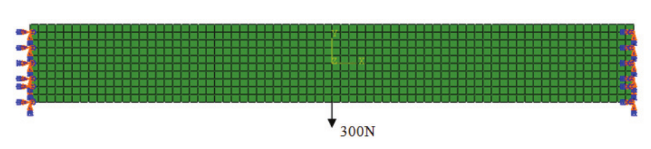
Figure 1.
Initial project domain for a transient analysis.
The initial parameters used for optimization are as follows: RR0= 10% and ER = 0.5%, with cavity control to open a maximum of five holes during the evolutionary process. A high initial rejection ratio was adopted owing to the non-removal of elements for lower values, and for this reason, a good element removal process can be obtained. In this example, the structure should be optimized until a volume fraction of 50% is removed.
To evaluate the influence of the damping ratio on the optimization, two types of analyses should be conducted, a linear analysis and a physical and geometric non-linear analysis. For both cases, an undamped model is considered, as are two additional models with different damping ratios assigned to the material, i.e., damping ratio A ( ) for values of
  and
and  , and damping ratio B (
 ) for
) for  and
and  .
.
To ensure that the adopted coefficients correspond to the underdamped case, which denotes an oscillatory movement, a modal analysis of the initial geometry was conducted to obtain the first natural frequency of the structure, the first vibration mode of which is shown in Figure 2.
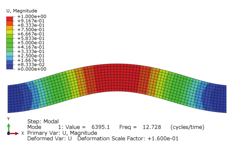
Figure 2.
First vibration mode of the initial geometry applied to the optimization studies for damping ratios A and B.
Thus, the respective damping ratios A and B based on the first vibration
mode can be obtained according to Equations 15 and 16 for the mass and
stiffness adopted portions as the analysis parameters, and the fundamental
frequency,  , was determined through a modal analysis.
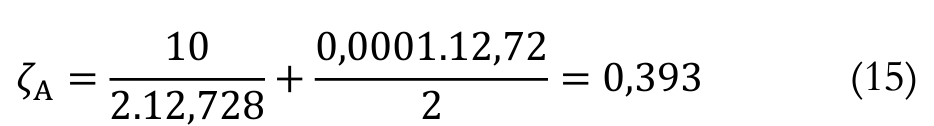 (15)
(15)
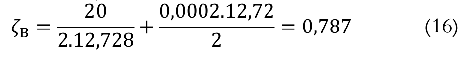 (16)
(16)Therefore, it is possible to ensure that oscillatory
movement occurs because the damping ratios are found to be within the range of  .
.
The calculation method used for this type of analysis corresponds to an implicit convergence approach because the represented problem corresponds to a long-term scenario, which is almost similar to a static solution characterized as a quasi-static problem. Another relevant factor is the use of a simple model with few degrees of freedom, enabling an inversion of the matrix proportional to the mass, damping, and stiffness.
Linear dynamic analysis
In the first structural optimization example, it is possible to verify the optimal topology obtained for the undamped linear dynamic analysis according to Figure 3.
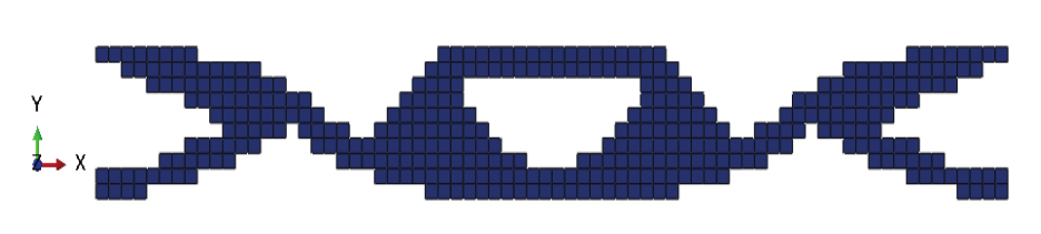
Figure 3.
Optimal topology for the undamped linear dynamic analysis.
The structural optimum design obtained through the corresponding ESO method for a transient dynamic analysis is very similar to the final result by Jung and Gea (2004), although its solution refers to a static condition. This clearly occurs because the dynamic action in this study is first applied using a slow load rate.
The similarity of Jung and Gea’s (2004) final topology is shown in Figure 4.

Figure 4.
Optimal topology obtained by Jung and Gea’s solution for a linear analysis under static loading condition. Source: adapted from Jung and Gea (2004).
Based on Figure 5, it is possible to verify the displacements of the load application node over time as a sinusoidal curve because there is no influence of damping.
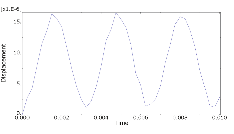
Figure 5.
Displacements of the load application node over time to the optimized geometry for the undamped linear model.
For the case involving the application of damping ratio A, the optimal topology obtained is as shown in Figure 6.
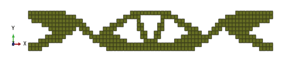
Figure 6.
Optimum topology for a linear dynamic analysis with damping ratio A.
To validate the results obtained by the optimization performed by ESO methodology considering the damping ratio ‘A’. It was run an additional optimization study in the commercial software Tosca® by using the Controller methodology, as well as the ESO methodology penalizes the elements in such a binary form not applying intermediate densities to the least efficient elements. The implementation of this methodology is based on an article by Sigmund (2001), in which the material distribution is applied according to the total strain energy of the model, and thus the volume is used as a restriction, and the minimization of the compliance is applied as an objective. The final topology obtained through this solution is as shown in Figure 7.
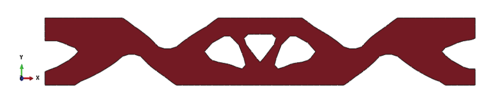
Figure 7.
Optimal topology obtained by Tosca® for a linear dynamic analysis with damping ratio A.
It is worth noting that stresses along the iterative process do not necessarily occur in the same element, providing a global aspect to the optimization. In this analysis, the stresses are concentrated in regions close to the load application.
Figure 8 shows the displacements of the load application node over time for the optimized geometry corresponding to damping ratio A. Therefore, a smoothing curve owing to the damping effect can be seen, minimizing the oscillatory motion.
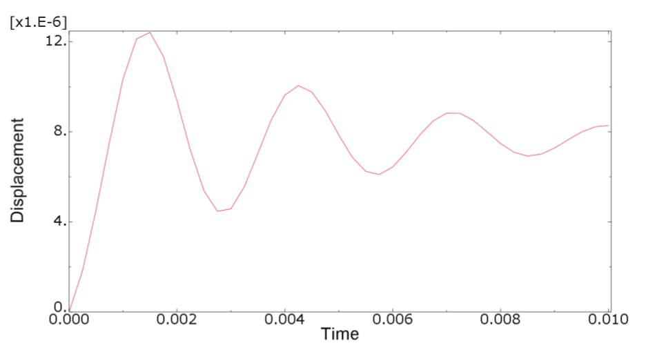
Figure 8.
Displacements of the load application node over time in the optimized geometry for the linear model with damping ratio A.
For the case involving the application of damping ratio B, the optimum topology obtained is as shown in Figure 9.
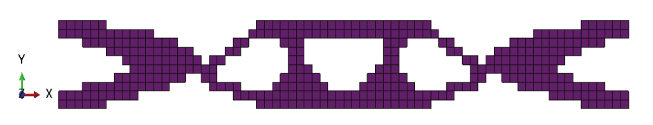
Figure 9.
Optimum topology for a linear dynamic analysis with damping ratio B.
In the same manner, for a model optimization using damping ratio A, an additional optimization study was applied to the model when considering damping ratio B through Tosca® software to validate the results obtained through the ESO methodology, as shown in Figure 10.
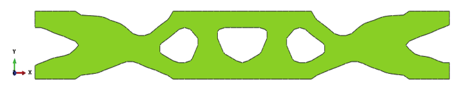
Figure 10.
Optimal topology obtained using Tosca® for a linear dynamic analysis with damping ratio B.
Figure 11 shows the displacements of the load application node over time for the optimized geometry corresponding to damping ratio B. For this condition, it is possible to realize a reduction in oscillatory motion relative to the previous one because there is a significant increase in the damping ratio.
According to the different solutions obtained for models with their respective damping ratios A and B, a response based on a combination of their final topologies can be considered, as shown in Figure 12.
To ensure that this evolutionary process optimizes the structure, an optimization rate was created. This rate consists of the relation between the volume fractions removed for each maximum level of von Mises equivalent stress obtained when considering all finite elements involved in the analysis. This maximum von Mises stress can occur for a different finite element during the evolutionary process, providing a global performance for the structural optimization.
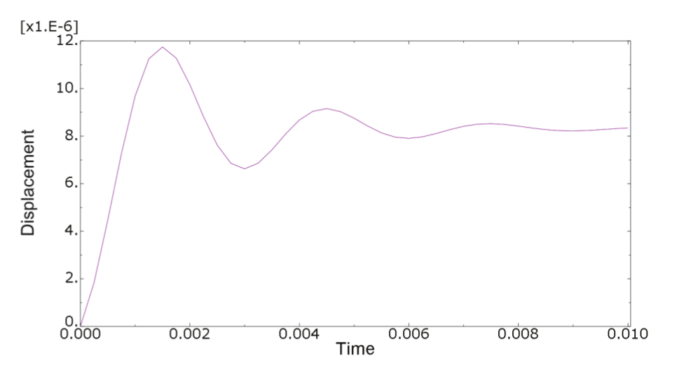
Figure 11.
Displacements of the load application node over time for the optimized geometry of the linear model with damping ratio B.
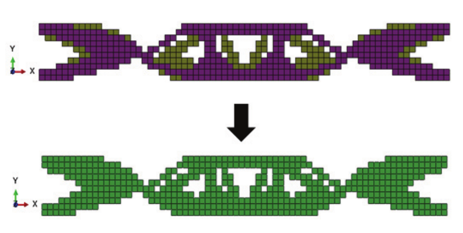
Figure 12.
Optimal topology for the combined effect of damping ratios A and B, considering a linear behavior.
The optimization rates for each iteration for the three damping conditions addressed for the linear elastic model are shown in the curves of Figure 13, and in this way it is possible to ensure that the evolutionary process optimizes the structure.
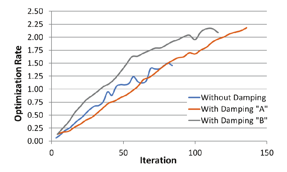
Figure 13.
Rate of evolutionary optimization process for each iteration of the linear elastic model.
Using such graphs, it is possible to check the best optimization stages for each damping ratio considered, and to show the best optimization points throughout the process.
Nonlinear dynamic analysis
For structural optimization with nonlinear behavior, a model with geometric nonlinearity was adopted in the elastoplastic regime, which will be simulated through a von Mises yield model when considering a material with linear isotropic work-hardening. The elastoplastic properties were taken generically, where the yield stress is represented as  KPa and the hardening modulus is represented as
  KPa. According to Li et al. (2014), the plastic behavior of ductile materials can be also represented by a combination between isotropic and plastic hardening modules.
In the same way presented for the example of linear behavior, three models will be considered, two of which have different damping ratios A and B, and the other has no damping application. Through Figure 14, it is possible to check the optimal topology obtained for an undamped dynamic analysis when applying nonlinear behavior.
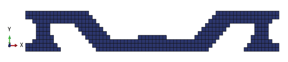
Figure 14.
Optimum topology for undamped nonlinear dynamic analysis.
The optimum structural design obtained by the ESO method for this nonlinear analysis is also similar to the solution obtained by Jung and Gea (2004) even under different loading condition, as shown in Figure 15.

Figure 15.
Optimal topology obtained using Jung and Gea’s solution for a nonlinear analysis under a static loading condition. Source: adapted from Jung and Gea (2004).
From Figure 16, it is possible to see a significant change in relation to the linear model for a displacement of the load application node over time owing to the influence of the elastoplastic properties during the yield phase.
For the case involving the application of damping ratio A, the optimum topology obtained is presented in Figure 17.
As with the example of the previous linear model, to validate the results obtained from the ESO method for damping ratio A, an additional optimization study was conducted using the commercial software Tosca®, the final topology of which is shown in Figure 18.
Figure 19 shows the displacements of the load application node over time for the optimized geometry corresponding to damping ratio A. It is possible to see a minimization of the displacement owing to the damping effect.
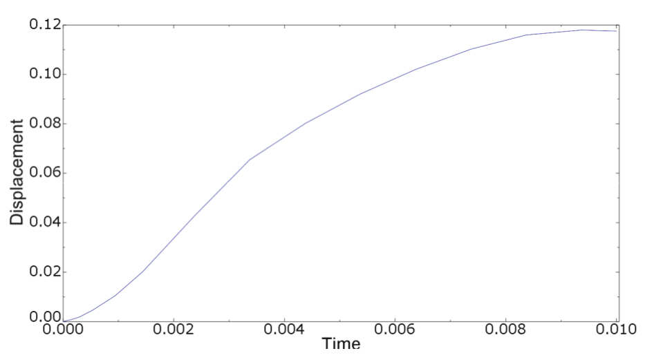
Figure 16.
Displacements of the load application node over time for an optimized geometry for the undamped nonlinear model .
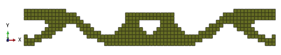
Figure 17.
Optimal topology for a nonlinear dynamic analysis with damping ratio A.
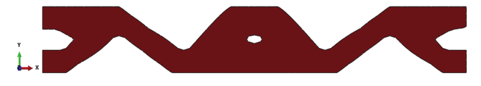
Figure 18.
Optimal topology obtained using Tosca® for nonlinear dynamic analysis with damping ratio A.
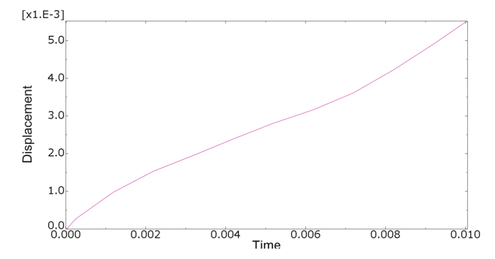
Figure 19.
Displacement of the load application node over time for the optimized geometry of the nonlinear model with damping ratio A.
For the case involving the application of damping ratio B, the optimum topology obtained is as shown in Figure 20.
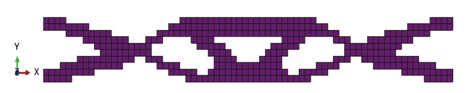
Figure 20.
Optimal topology for nonlinear dynamic analysis with damping ratio B.
In the same way as applied for the model optimization with damping ratio A, an additional optimization study was conducted for the model with damping ratio B using Tosca® software to validate the results obtained through the ESO methodology, as shown in Figure 21.
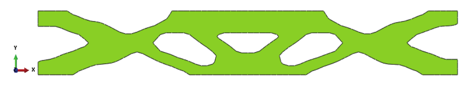
Figure 21.
Optimal topology obtained using Tosca® for nonlinear dynamic analysis with damping ratio B.
Figure 22 shows the displacements of the load application node over time for the optimized geometry corresponding to damping ratio B. For this condition, it is possible to see a small increase in displacement when compared to the previous one, even with a significantly increasing damping ratio.
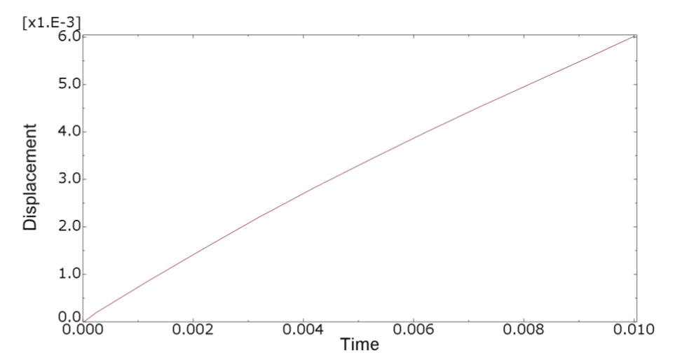
Figure 22.
Displacement of the load application node over time for the optimized geometry of the nonlinear model with damping ratio B.
When applying the elastoplastic models, it is very important to verify that, as the damping ratio increases, the displacement curve over time tends to approach a static response curve, and becomes nearly linear. Otherwise, without material nonlinear behavior consideration, signifficant differences are observed between linear and geometric nonlinear optimum solutions (Fernandes et al., 2015).
According to the different solutions obtained for models with their respective damping ratios A and B, it is possible to consider a response based on a combination of the final topology of each model, as shown in Figure 23.
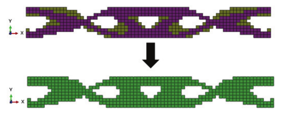
Figure 23.
Optimal topology for the combined effect of damping ratios A and B, considering nonlinear behavior.
As mentioned earlier, it is important to analyze the optimization rate for each iteration, as shown in the curves of Figure 24, for the three damping conditions addressed for the nonlinear model, thereby ensuring that the evolutionary process optimizes the structure.
The next step of the present study is to minimize sensitivity to uncertainties, which is the subject of the robust topological optimization (Zhao et al., 2015).
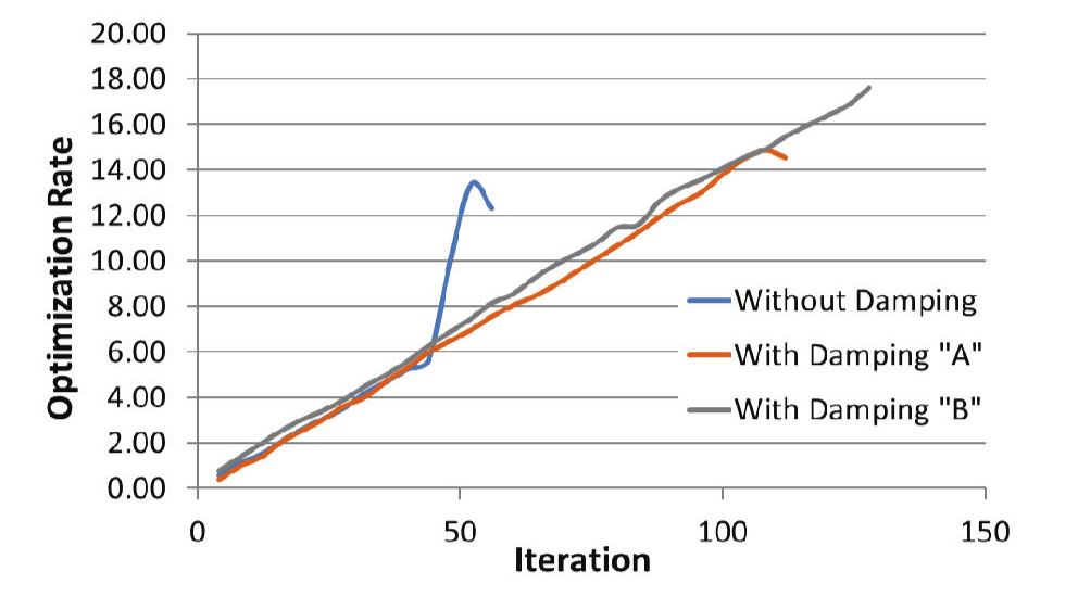
Figure 24.
Optimization rate of the evolutionary process for each iteration of the nonlinear model.
Conclusion
This evolutionary process has been shown to be capable of performing a routine in which it is possible to obtain a directional of the optimum disposition and the structural shape under dynamic conditions.
The proposed work used various resources available in the commercial software Abaqus®, which enables structural analyses requested through either static or dynamic actions to be conducted with or without nonlinearity.
According to the results, a modification of the damping ratio can cause significant changes in the structural stiffness, mainly for elastoplastic problems, as can be seen through the displacement curves over time, which consequently brings about changes in the structural stress levels.
Acknowledgements
The authors acknowledge the financial supports granted by CNPq (Conselho Nacional de Desenvolvimento Científico e Tecnológico), CAPES (Coordenação de Aperfeiçoamento de Pessoal de Nível Superior) and FAPEMIG (Fundação de Amparo à Pesquisa do Estado de Minas Gerais).
References
Bendsøe, M. P., & Sigmund, O. (2003). Topology optimization: theory, methods and application. Berlin, DE: Springer-Verlag.
Fernandes, W. S., Greco, M., & Almeida, V. S. (2017). Application of the smooth evolutionary structural optimization method combined with a multi-criteria decision procedure. Engineering Structures, 143(1), 40-51.
Fernandes, W. S., Almeida, V. S., Neves, F. A., & Greco, M. (2015) Topology optimization applied to 2D elasticity problems considering the geometrical nonlinearity. Engineering Structures, 100(1), 116–127.
Huang, X., & Xie, M. (2010). Evolutionary topology optimization of continuum structures: methods and applications. Chichester, UK: Wiley.
Jung, D., & Gea, H. C. (2004). Topology optimization of nonlinear structures. Finite Elements in Analysis and Design, 40(11), 1417-1427.
Kim, H., Querin, O. M., Steven, G. P., & Xie, Y. M. (2002). Determination of an optimal topology with a predefined number of cavities. AIAA Journal, 40(4), 739-744.
Lanes, R. M., & Greco, M. (2013). Aplicação de um método de otimização topológica evolucionária desenvolvido em script python. Science & Engineering, 22(1), 1-11.
Li, R., Zhang, Y., & Tong, L. (2014). Numerical study of the cyclic load behavior of aisi 316 stainless steel shear links for seismic fuse device. Frontiers of Structural and Civil Engineering, 8(4), 414-426.
Maute, K., Schwarz, S., & Ramm, E. (1998). Adaptive topology optimization of elastoplastic structures. Structural Optimization, 15(2), 81-91.
Oliveira, F. M., & Greco, M. (2014). Nonlinear dynamic analysis of beams with layered cross sections under moving masses. The Brazilian Society of Mechanical Sciences and Engineering, 37(2), 451-462.
Ramm, E., & Matzenmiller, A. (1988). Consistent Linearization in elastoplastic shell analysis. Engineering Computations, 5(4), 289-299.
Sigmund, O. (2001). A 99 line topology optimization code written in Matlab. Structural and Multidisciplinary Optimization, 21(2), 120-127.
Simo, J. C., & Hughes, T. J. R. (1998). Computational inelasticity. New York City, NY: Springer-Verlag.
Tanskanen, P. (2002). The evolutionary structural optimization method: theoretical aspects. Computer Methods in Applied Mechanics and Engineering, 191(47-48), 5485-5498.
Xie, M. Y., & Steven, G. P. (1993). A simple evolutionary procedure for structural optimization. Computer & Structures, 49(5), 885-896.
Xie, Y. M., & Steven, G. P. (1997). Evolutionary structural optimization. London, UK: Springer-Verlag.
Zhao, Q., Chen, X., Ma, Z., & Lin, Y. (2015). Robust topology optimization based on stochastic collocation methods under loading uncertainties. Mathematical Problems in Engineering, Article ID 580980. doi: 10.1155/2015/580980
Notes
Author notes
mgreco@dees.ufmg.br