Introduction

From the Constructal Law (Bejan & Zane, 2012), the geometrical configuration of a finite-size flow system must evolve to ease the access of the currents that flow through it, otherwise, it will not persist in time. Following this principle, the design in engineering has to begin discovering the flow architecture that facilitates flow access between a point source and a volume, and vice versa. Observing the evolutionary designs which improve flow access in nature, they have turned to be dendritic. Bearing in mind that this is not result of chance, the so-called Constructal Design has been used to discover the best geometrical shapes for different applications in heat transfer (Biserni, Rocha, Stanescu, & Lorenzini, 2007; Lorenzini et al., 2013), fluid mechanics (Reis, 2006; Cetkin, Lorente, & Bejan, 2010) and convection heat transfer (Rocha, Lorente, & Bejan, 2009; Kim, Lorente, & Bejan, 2010), just to mention a few.

Therefore, the Constructal Design can be very useful to help finding the optimal geometry arrangements which enhance the energy performance of Earth-Air Heat Exchangers (Eahe). Eahe are sets of fans and buried ducts that take advantage of the thermal inertia of the superficial layers of soil, since it presents lower temperatures than the external air during summer and vice versa in the winter. Hence, the fans blow the air inside the ducts (from the constructal point of view: the ‘point source’), where it exchanges heat with the surrounding soil (the ‘volume source’), and comes out inside a building or house at a milder temperature, thus saving electrical energy for air conditioning (Brum, Rocha, Vaz, Santos, & Isoldi, 2012; Vaz, Sattler, Brum, Santos, & Isoldi, 2014). That said, an important question to design better Eahe is posed in the Figure 1. How one should arrange the ducts to improve the Eahe performance? So far, related questions have been pursued in several works, e. g. (Rocha, Lorent, Bejan, & Anderson, 2012; Rodrigues et al., 2015).

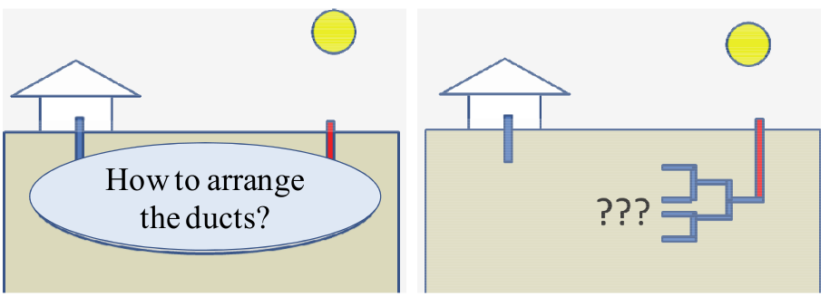
Figure 1.
Design question for Eahe.

This paper addresses some of these questions through the case study of Eahe composed by three ducts and using the method of constructal design, which consists of morphing freely the flow configuration towards the direction of the main currents that flow through it subjected to constraints (volumes). Here, the current is heat, and it flows between the ducts and the ground. As in (Rodrigues et al., 2015), the ducts assembly is assumed to occupy a constant volume V_EAHE whose center is buried at a depth D_aveinside a portion of soil with constant volume V_s. It is assumed that the Eahe volume takes the shape of a triangular prism while the soil is a parallelepiped. Two spacings among the ducts are considered: a horizontal S_h and a vertical one S_v, which are free to vary under constraints, such as a fixed volume fraction , which is the ratio between V_EAHE and V_s. Then, the general objective is to understand how the heat exchange varies (or is maximized) as the structure evolves assuming different values for the ratio s = S_h / S_v.

As it is shown ahead, from the values of the temperature fields on the ducts inlets and outlets, averages of their differences, called thermal potentials of Eahe are computed. This work presents new models for the thermal potentials in function of the ratio s . Among other results, this allows to establish important findings, from the constructal point of view, such as the best shape for the ducts assembly.

Material and methods

This study assesses the performance of many different geometrical arranges of three ducts buried in a three-dimensional portion of soil with height H_s = 15 m, width W_s= 10 m and length L_s = 26 m, as illustrated by Figure 2a. Each duct is a right circular cylinder with length $l$ = 26, and diameter d = 0.127 m. Furthermore, their centers are placed at the corners of an isosceles triangle around a fixed center point 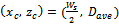, as in the Figure 2b. Here, D_ave= 3 m which is the depth recommended by previous researches (Brum et al., 2012) for Eahe with only one duct, considering experimental data obtained in the Brazilian city of Viamão (Vaz et al., 2014). From Figure 2b, one also notices that ($\textcolor{red}{}xc$, $\textcolor{red}{}zc$) is the center of a rectangle whose base and height measure, respectively, S_hand S_v. These numbers represent the horizontal and vertical spacings among the ducts.

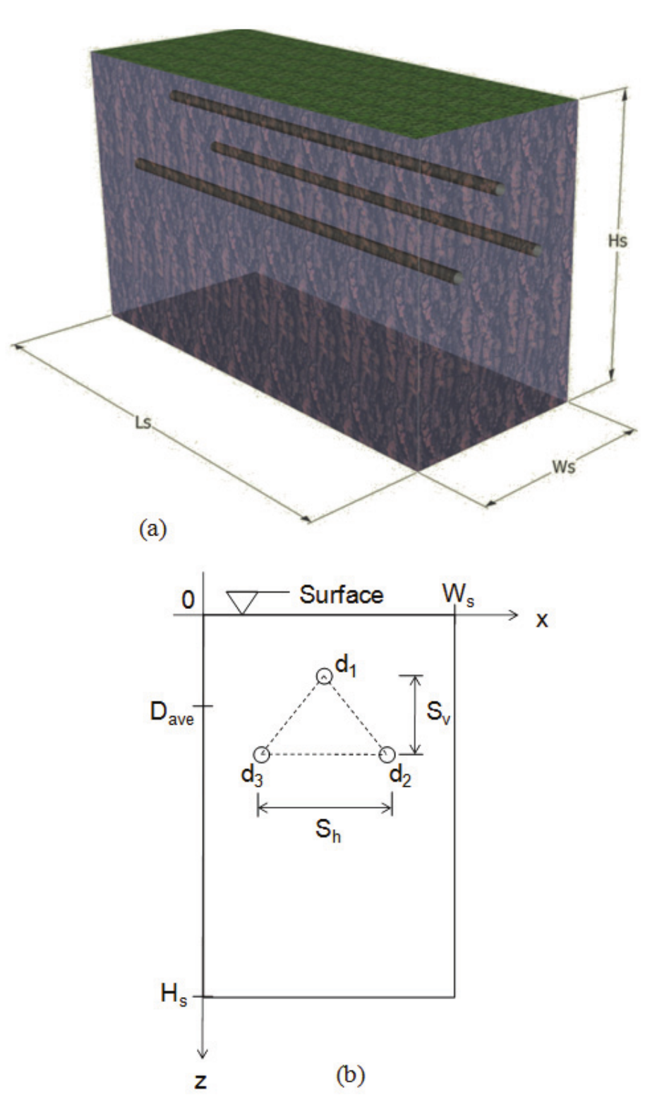
Figure 2.
(a) Soil and ducts three-dimensional view; and (b) Cross section view.

Basically, one objective here is to understand how the differences between the air temperatures on the outlet and inlet sides of the ducts are maximized as the triangular shape of the arrangements vary. More specifically, the degree of freedom is the ratio between S_h and S_v, subject to fixed constraints: the volume occupied by the Eahe V_EAHE and the volume of the soil considered V_s. The V_EAHE constraint can be replaced by the volume fraction , i.e., the ratio between V_EAHE and V_s. Three-dimensionally speaking, the Eahe is assumed to be a triangular prism and the soil a parallelepiped, then is defined by Equation 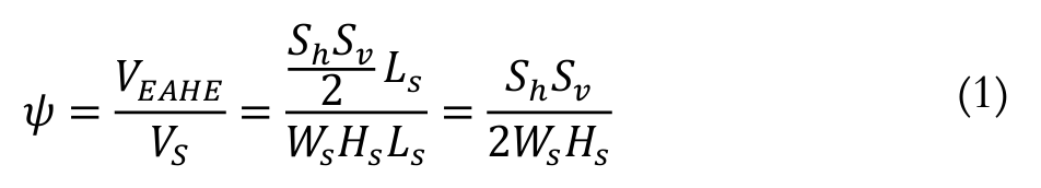1:

(1)

Since the ducts cannot intersect and they have to be inside the soil, it should be imposed further constraints, which are: S_h > d, S_v > d, S_h < W_s – 2 d, S_v < 2 D_ave - 0.5. As it has been done in related studies (Rodrigues et al., 2015), this research considered many different ratios S_h/S_vfor three different volume fractions, whose values are properly summarized in the next section.

To simulate numerically the temperature fields, the computational domain was constructed and discretized using the Gambit software. The solution of governing equations and post-processing were done with the Fluent software which employs the finite volume method. All cases employed tetrahedral cells whose quantity varied around 33000 and 720000 for the ducts and the soil regions, respectively. The mesh was more refined in the ducts to improve precision. In the soil, the cells could have a maximal interval size of 10d/3. These numbers came from mesh independence tests performed in previous research (Rodrigues et al., 2015). To avoid unnecessary complications, the ducts were simply assumed to be cylindrical perforations in the soil, i. e., their thickness and material properties were neglected. This simplification has already been adopted in many studies (Brum et al., 2012; Brum, Isoldi, Santos, Vaz, & Rocha, 2013a; Brum, Vaz, Rocha, Santos, & Isoldi, 2013b; Vaz et al., 2014; Rodrigues et al., 2015) since it was previously validated against experimental data. Regarding time discretization, all simulations used a time step of 3600 s, with a maximum of 200 interactions per time step, covering a total period of two years.

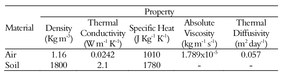
This study also considered the experimental data from (Vaz et al., 2014) to represent the air and clay soil from the Brazilian city of Viamão, whose thermo-physical properties are assembled in Table 1. Furthermore, using the least squares method as in (Brum, Ramalho, Rocha, Isoldi, & Santos, 2015), the soil surface and air temperatures along one year in that city were modeled, respectively, by the Equation 2 and 3:

Table 1.

Thermo-physical properties of Air and Soil.

(2)

(3)

where:

The temperatures are in ⁰C and the time t in days. Hence, these equations were used, in this order, to impose boundary conditions for the temperature on the upper surface of the computational domain and at the inlet of each duct. Also at the inlet, it was imposed a velocity of 1.0 m s^-1. At the outlet it was prescribed the atmospheric pressure. As for the other surfaces, they were considered thermally insulated. For the initial condition, the temperature in all domain is considered equal to the soil mean temperature, i. e., 18.70⁰C.

The simulations involved a very complete computational model for Eahe (Brum et al., 2012; Brum et al., 2013b; Vaz et al., 2014). Except for the soil, where the evaluation of the transient temperature field considers only the conservation equation of energy, inside the ducts the time-averaged conservation equations of mass, momentum and energy (Wilcox, 2002; Versteeg & Malalasekera, 2007) were used to model a transient, incompressible, turbulent forced convective flow. The Reynolds Stress Model (RSM) was used to deal with the turbulence; for the treatment of transient pressure and velocity fields it was used the Coupled algorithm; to handle numerical instabilities from the advection terms of conservation equations of momentum and energy, as well as, for equations of the closure model, it was employed the upwind scheme. Finally, the results were considered converged when the residuals for mass, momentum, and energy between two consecutives iterations were lower than 10^-3, 10^-3 and 10^-6, respectively.

Results and discussion

Modeling the instantaneous thermal potential

Many studies (Brum et al., 2012; 2013a; 2013b; Vaz et al., 2014; Rodrigues et al., 2015) analyze Eahe by a performance criteria called thermal potential P_T, which is often defined simply by the time average of the differences between the air temperatures on the outlet and inlet sides of the ducts.

This paper formally defines the P_T further ahead after developing other important concepts. First, for Eahe with q ducts, let d_k be the difference between the air temperatures on the outlet T_o,kand on the inlet T_i,k of the k-th duct in the time t, that is, by Equation 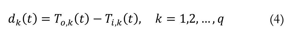4:

(4)

Thus, let the instantaneous thermal potential P be defined by the mean of the q temperature differences, which is in the Equation 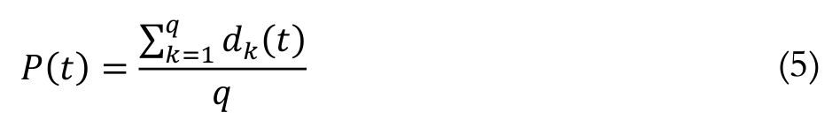5:

(5)

Indeed, for Eahe arrangements similar to the one shown in Figure 2, P is a function of many variables besides time. However, from the perspective of the constructal design (Bejan & Lorente, 2008; Rodrigues et al, 2015) there is a particular interest to understand the relationship between the thermal potential and the geometrical degrees of freedom S_h and S_v, which represent, respectively, the horizontal and vertical spacings among the ducts.

A major contribution of this paper is to find that P can be written in the form of Equation 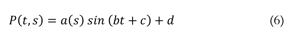6:

(6)

where:

s = S_h/S_v, b, c and d are real constants, a is a function of s, and t stands for time, as before. In physical terms, it is usual to say that: a represents the potential amplitude, b its angular frequency, c the phase, and d the mean value. As it is shown later, this means that the intensity of the thermal potential of Eahe is directly related to s.

It has already been noticed in previous studies (Vaz et al., 2014; Brum et al., 2015) that the temperatures on the inlet and outlet of Eahe have a periodical behavior well captured by sine based functions. Even though works e. g. (Rodrigues et al., 2015) have studied some correspondence between and the thermal potential, they have not attempted to model their relationship. As shown in Figure 3, where there is a comparison of the instantaneous thermal potential P for three different values of s, under the same volume fraction , the fraction s influences directly the amplitudes, hardly changing their frequency, phase, or mean value.

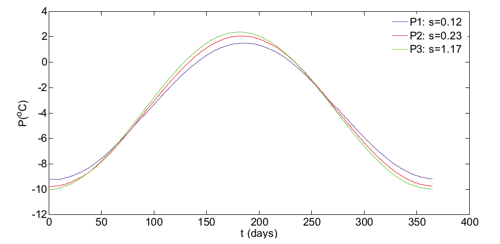
Figure 3.
Three cases of thermal instantaneous potentials along one year for u = 0.01 .

To further verify this hypothesis, it was first considered individually m different cases of ratios s = S_h/S_v for the same volume fraction . Then, the instantaneous thermal potentials were modeled in the form of Equation 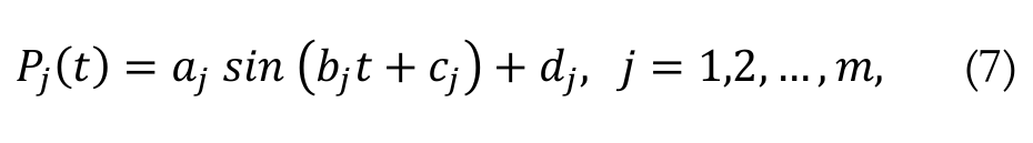7:

(7)

where:

a_j, b_j, c_j, and d_jare real coefficients which are determined by the least squares method as in (Brum et al., 2015).

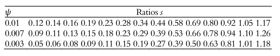
The Table 2 presents the approximate values of for the corresponding volume fractions = 0.01, 0.007 and 0.003. Hence, for each value of it was considered m = 14 different values of s.

Table 2.

Values of s = S_h/S_v for u = 0.01, 0.007 and 0.003.

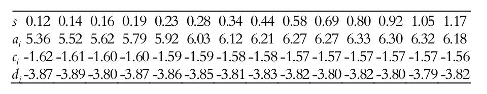
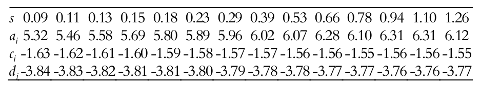
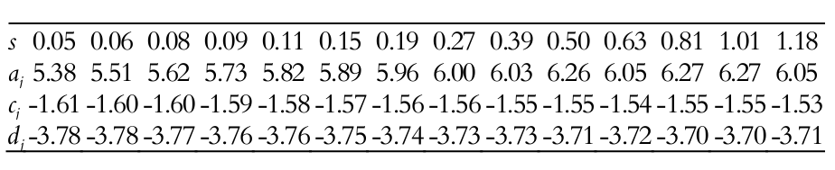
Regarding the values of the coefficients a_j, c_jand, d_j all of them are presented, approximately, in the Table 3, 4 and 5, considering the volume fractions = 0.01, 0.007 and 0.003, respectively. Since the instantaneous thermal potential is periodic, and its period is one year, then b_j should be equal to , because it represents the angular frequency, and the year was simulated with 365 days. Thus, as expected, for all cases, the numerical results gave .

From the Table 3 to 5, the coefficients c_jand d_j relatively vary much less than a_jwith respect to the variable s. For example, taking = 0.007, the standard deviations (Bulmer, 1979) of a_j, c_j and, d_j are 0.32, 0.03 and 0.03, respectively. In all cases, the standard deviations for b_j were negligible. Therefore, it is very reasonable to approximate the coefficients b_j, c_j and, d_j by their respective mean values and only obtain a classical polynomial fitting, by least squares (Gerald & Wheatley, 2004), to the coefficient a_j as a function of s.

Table 3.

Values of the coefficients a_j, c_j and, d_j for each s considering u = 0.01.

Table 4.

Values of the coefficients a_j, c_jand, d_j for each s considering u = 0.007

Table 5.

Values of the coefficients a_j,c_j and, d_jfor each s considering u = 0.003.

All things considered, for the temperature fields obtained numerically, it is possible to develop the following three functions to model the instantaneous thermal potential.

For = 0.01, Equation 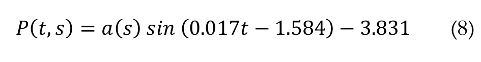8:

(8)

where, Equation 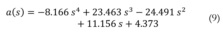9:

(9)

For = 0.007, Equation 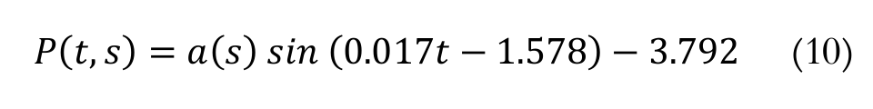10:

(10)

where, Equation 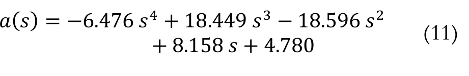11:

(11)

For = 0.003, Equation 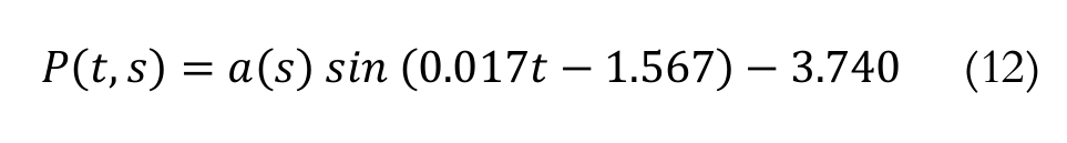12:

(12)

where, Equation 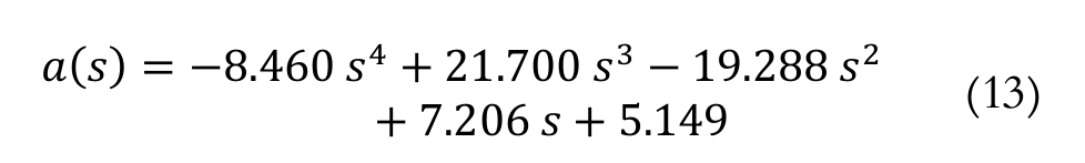13:

(13)

In all these equations, the units for P and t are, respectively, ⁰C and days. The variable s is dimensionless. Here, it is important to highlight that the fourth degree polynomials were adopted to increase precision. The Figure 4 compares the graphics of the discrete results a_j and its three fitting polynomials of degree 4, 3 and, 2 respectively named: a₄(s), a₃(s) and a₂(s). As shown, a4(s) follows the data more closely. In fact, for this case, there is a Pearson’s R correlation coefficient (Bulmer, 1979) among a₄ (s_j) and a_j of 0.997.

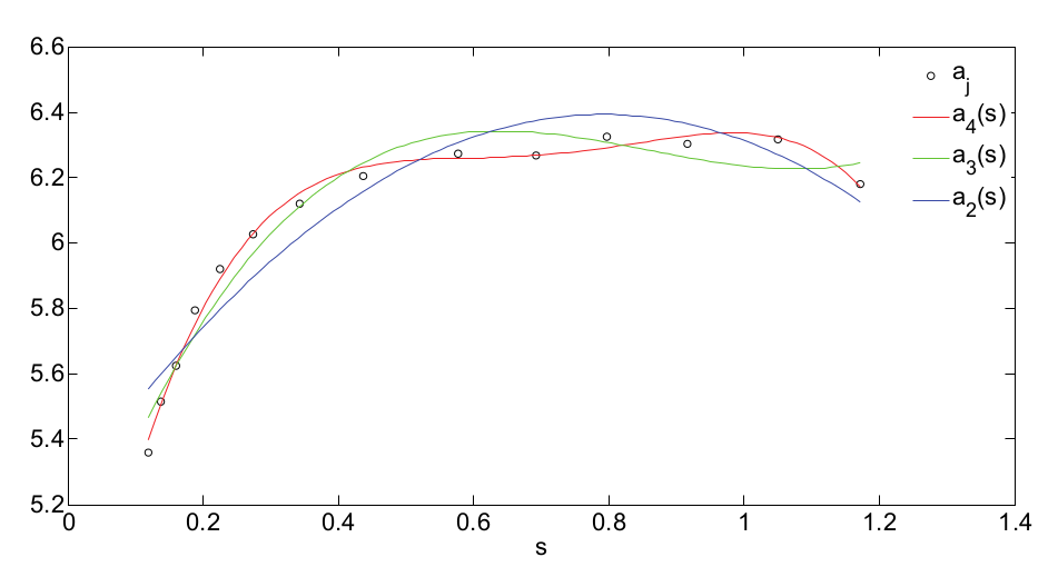
Figure 4.
Comparison between aj and its fitting polynomials an (s) of degree n for u = 0.01.

For Eahe projects, a main objective is to maximize the differences (positive or negative) between the temperatures on the ducts outlet and inlet. Therefore, it is very important to compute the maximum and minimum of the instantaneous thermal potential functions.

Hence, using these newly developed function, one first step is to find the maximum amplitude of the instantaneous potential which is given by the functions a(s). Since these functions are polynomials, their maximum values occur where their first derivatives are zero, or at the boundaries of the intervals considered for the variable s (Stewart, 2006).

In the case of = 0.01, s varies in the interval [0.12, 1.17]. The derivative of a(s) is given by Equation 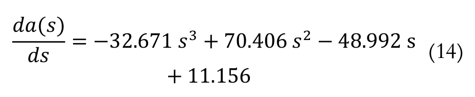14:

(14)

which is zero, approximately, at s = 1. Since a(0.12) = 5.40, a(1.00) = 6.34 and a(1.17) = 6.17, then it is possible to conclude that the maximal amplitude of the instantaneous thermal potential is approximately 6.34⁰C which occurs for a relation .

Making similar computations for = 0.007 and = 0.003, the maximal amplitude also occurs when , changing only its values for 6.31⁰C and 6.31⁰C, respectively. Thus, from these comparisons, the volume fraction = 0.01 gives the best thermal performance for the cases considered in this paper.

Looking at these results from the geometrical aspect, they also represent a contribution to the Constructal Theory (Bejan, 1997; Bejan & Lorente, 2008). An important question for the design of Eahe is how to find the flow architecture (ducts spacings and shapes of their arrangements) which increases the heat exchange with the soil. In this sense, it is possible to interpret the set of simulations presented here as an analysis of the evolution of Eahe (particularly, its instantaneous thermal potential P ) under free changes in its flow configurations (horizontal and vertical spacings: s) up to limiting constraints. At the end, inside the variation of volume fractions ) studied, one finds out that robust arrangements for the ducts take the shape of isosceles triangles with unitary base and height. This goes along with the results of a related study (Rocha et al., 2012), where it is found that the best shapes for sets of four heat pumps tend to squares, for similar ranges of volume fractions also adopted in this paper.

After computing the maximum value of the amplitude as a function of s, it is possible to find the maximum and minimum values of the instantaneous thermal potential relatively to the time t. In particular, it is convenient to focus the analysis, from here on, considering = 0.01 and the potential function defined by the Equation 8 and 9, since the higher amplitude was achieved for this volume fraction.

Therefore, as the maximum and minimum values of the sine function are, respectively, and - , they occur at the following days. Maximum: Minimum: .

As expected, these results agree with the graphics in Figure 3, where the maximum value of the instantaneous thermal potential occurs almost at the middle of the year (after days, during the winter) while its minimum value occurs at the beginning of the year (in the summer). Based on these data, the maximum and minimum values for the instantaneous thermal potential, for all cases studied, are given by Equation 15 and 16:

(15)

(16)

Thermal potential

Given these results, it is all set to define the so-called thermal potential P_T used in many references (Brum et al., 2012; 2013a; 2013b; Vaz et al., 2014; Rodrigues et al., 2015) from the concept of the instantaneous thermal potential P, introduced in this paper. In general, the P_T in these studies can be seen as monthly mean values of P.

Considering the numerical simulations, adopting a fixed value for the ratio s, the months can be discretized in n + 1 times t₀, t₁, …, t_n equaly separated by intervals of size . Thus, the monthly thermal potential can be computed by the Equation 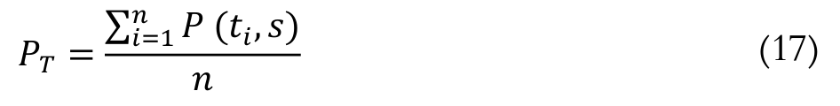17:

(17)

which is equivalent to Equation 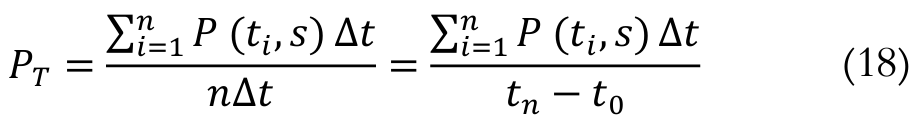18:

(18)

Hence, continuously speaking, if , the thermal potential can be formally defined by Equation 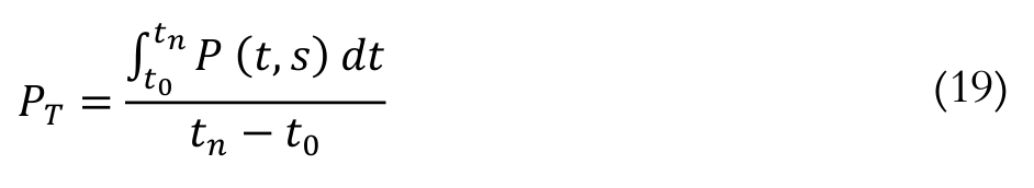19:

(19)

for each fixed value of s.

From these analyses, the highest thermal potential for cooling is achieved in January (from the day 0 to 31) for a ratio s = 1. Furthermore, it is given by Equation 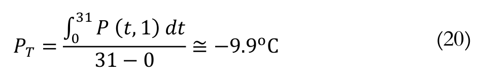20:

(20)

On the other hand, the highest thermal potential for heating occurs in July (among the days 181 to 212) and it is given by Equation 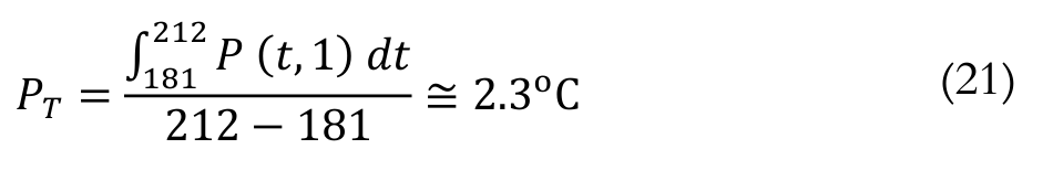21:

(21)

Eahe’s efficiency

Although the thermal potential gives one way to compare different arrangements of Eahe, it is not a dimensionless quantity and it does not offer a clear measure of efficiency. In this regard, one can use the temperature ratio (Pfafferott, 2003), defined by Equation 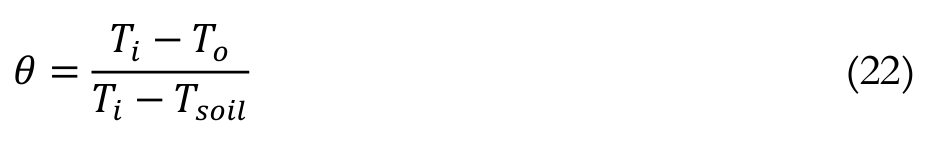22:

(22)

where:

T_i and T_o are the temperatures on the inlet and on the outlet of the ducts, respectively, while T_soil is the soil temperature.

In this study, it is computed an average of the temperature ratio along intervals of days [c, d], through the Equation 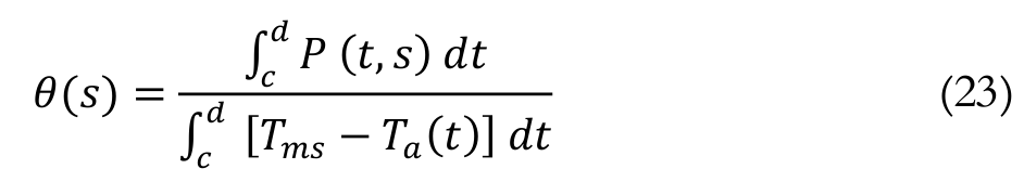23:

(23)

where:

P (t, s) is the instantaneous thermal potential defined in Equation 8 and 9; Tms = 18.7⁰C, which is the mean temperature of the soil at the center of the Eahe installations, i.e., at the point (x, z) = (W_s /2, D_ave), relatively to Figure 2b; T_a(t) is the temperature of the air on the ducts inlet, which is given in Equation 3.

Ideally, should be a scale unit because, at first sight, the absolute value of the differences between the temperatures on the outlet and inlet of Eahe should not be higher than the absolute value of the differences between the temperatures on the inlet and in the soil. Besides, if the heat exchange is perfect, the temperature on the outlet should be equal to the temperature in the soil. However, this is not true, particularly, in the spring and in the fall, when the air temperature can be equal to the soil temperature.

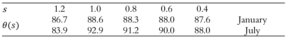
Thence, it is convenient to compute the Eahe efficiency at the peak of the Brazilian summer, in January, and at the peak of winter, in July. The Table 6 presents some results of efficiency in these months. As expected, the Eahe are more efficient when . To raise or reduce s around this value reduces the efficiency. Furthermore, the best performance for Eahe occurs in the winter, when they achieve 92.9% of efficiency.

Table 6.

Eahe efficiency (in %) in the months of January and July.

Energetic performance

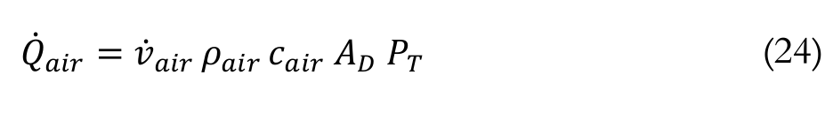
A final important concern regarding Eahe is to determine its heat transfer rate, or its monthly energy performance, which can be computed (for each duct) by the Equation 24 (Pfafferott, 2003):

(24)

where:

= 1 m s^-1, = 1.16 = Kg m^-3 and c_air = 1010J/(Kg K^-1) represent, respectively, the average velocity, the density and the specific heat of the air in the ducts; A_D = 0.0127 m² is the cross section area of the ducts; P_T is the thermal potential previously defined in Equation 19, computed over a month.

Therefore, considering the peak months, the volume fraction = 0.01 and the ratio s = 1, in average, the Eahe have a cooling power of 440.7 W in January and a heating power of 103,4 W in July. In energetic therms, this means 327.9 KWh in January and 77.0 KWh in July.

Conclusion

With the constructal design method, one examines the evolution of the thermal potential as the geometry of flow configuration varies in the direction of greater flow access for its currents. In this study, the current is heat, and it flows from the ducts of Eahe to the soil or vice versa. The objective is to determine the shape and spacing among the ducts which increase the heat exchange.

Based on constructal design, this paper introduces mathematical models to determine thermal potentials of Eahe composed by three ducts. Using the concept of instantaneous thermal potential P, which is an average of the differences between the air temperatures on the ducts outlets and inlets, this essay not only finds that P is periodic but also that its amplitude is affected directly by the ratio s between the ducts horizontal and vertical spacing.

This leads to new models for P in function of and the time t. From these models, inside the range of simulations studied, this paper finds: the best volume fraction for Eahe ( = 0.01); the maximal amplitude of P (6.34⁰C); the best spacing among the ducts (occurring for ); the best shape (the results point that the ducts should be arranged forming an isosceles triangle with unitary base and height); the days and months with higher potentials and its values (occurring in January and July). It also allows computing the Eahe efficiency in the best months of winter (92.9%) and summer (88.6%), and the energetic performance, which achieves a maximum of 327.9 KWh in January.

As a final remark, the methodology employed for the first time in this paper, to model the instantaneous thermal potential, considered only three ducts as a case study. Its applicability to analyze other cases and geometries with only two ducts, or more than three, should be the subject of forthcoming works.

Acknowledgements

R. da S. Brum thanks to CNPq for her doctoral scholarship. L. A. Isoldi thanks to CNPq (Process: 445558/2014-8). E. D. dos Santos, L. A. Isoldi and L. A. O. Rocha thank to CNPq for financial support.

References

Bejan, A. (1997). Advanced engineering termodynamics. New York City, NY: John Wiley & Sons.

Bejan, A., & Lorente, S. (2008). Design with constructal theory. Hoboken, NJ: John Wiley & Sons.

Bejan, A., & Zane, J. P. (2012). Design in nature. New York City, NY: Doubleday.

Biserni, C., Rocha, L. A. O., Stanescu, G., & Lorenzini, E. (2007). Constructal H-shaped cavities according to Bejan’s theory. International Journal of Heat and Mass Transfer, 50(11-12), 2132-2138.

Brum, R. S., Isoldi, L. A., Santos, E. D., Vaz, J., & Rocha, L. O. (2013a). Two-dimensional computational modeling of the soil thermal behavior due to the incidence of solar radiation. Engenharia Térmica (Thermal Engineering), 12(2), 63-68.

Brum, R. S., Ramalho, J. V. A., Rocha, L. A. O., Isoldi, L. A., & Santos, E. D. (2015). A Matlab code to fit periodic data. Revista Brasileira de Computação Aplicada, 7(2), 16-25.

Brum, R. S., Rocha, L. A. O., Vaz, J., Santos, E. D., & Isoldi, L. A. (2012). Development of simplified numerical model for evaluation of the influence of soil-air heat exchanger installation depth over its thermal potential. International Journal of Advanced Renewable Energy Research, 1(9), 505-514.

Brum, R. S., Vaz, J., Rocha, L. A. O., Santos, E. D., & Isoldi, L. A. (2013b). A new computational modeling to predict the behavior of earth-air heat exchangers. Energy and Buildings, 64, 395-402.

Bulmer, M. G. (1979). Principles of statistics. New York City, NY: Dover Publications Inc.

Cetkin, E., Lorente, S., & Bejan, A. (2010). Natural constructal emergence of vascular design with turbulent flow. Journal of Applied Physics, 107(11), 114901-114910.

Gerald, C. F., & Wheatley, P. O. (2004). Applied numerical analysis. Boston, MA: Pearson/Addison-Wesley.

Kim, Y., Lorente, S., & Bejan, A. (2010). Constructal multi-tube configuration for natural and forced convection in cross-flow. International Journal of Heat and Mass Transfer, 53(23-24), 5121-5128.

Lorenzini, G., Biserni, C., Link, F. B., Isoldi, L. A., Santos, E. D., & Rocha, L. A. O. (2013). Constructal Design of T-shaped cavity for several convective fluxes imposed at the cavity surfaces. Journal of Engineering Thermophysics, 22(4), 309-321.

Pfafferott, J. (2003). Evaluation of earth-to-air heat exchangers with a standardised method to calculate energy efficiency. Energy and Buildings, 35(10), 971-983.

Reis, A. H. (2006). Constructal view of scaling laws of river basins. Geomorphology, 78(3-4), 201-206.

Rocha, L. A. O., Lorente, S., & Bejan, A. (2009). Tree-shaped vascular wall designs for localized intense cooling. International Journal of Heat and Mass Transfer, 52(19-20), 4535-4544.

Rocha, L. A. O., Lorente, S., Bejan, A., & Anderson, R. (2012). Constructal design of underground heat sources or sinks for the annual cycle. International Journal of Heat and Mass Transfer, 55(25-26), 7832-7837.

Rodrigues, M. K., Brum, R. S., Vaz, J., Rocha, L. A. O., Santos, E. D., & Isoldi, L. A. (2015). Numerical investigation about the improvement of the thermal potential of an earth-air heat exchanger (Eahe) employing the constructal design method. Renewable Energy, 80, 538-551.

Stewart, J. (2006). Cálculo volume I. São Paulo, SP: Pioneira Thomsom Learning.

Vaz, J., Sattler, M., Brum, R. S., Santos, E. D., & Isoldi, L. A. (2014). An experimental study on the use of Earth-Air Heat Exchangers (Eahe). Energy and Buildings, 72, 122-131.

Versteeg, H. K., & Malalasekera, W. (2007). An introduction to computational fluid dynamics – the finite volume method. London, UK: Pearson Education.

Wilcox, D. C. (2002). Turbulence modeling for CFD. La Canada, CA: DCW Industries.

Notes

Author notes

jairo.ramalho@ufpel.edu.br