Estatística
Mathematical properties, application and simulation for the exponentiated generalized standardized Gumbel distribution
Mathematical properties, application and simulation for the exponentiated generalized standardized Gumbel distribution
Acta Scientiarum. Technology, vol. 41, 2019
Universidade Estadual de Maringá
Received: 01 October 2017
Accepted: 01 December 2017
Abstract: In this paper, we study the two-parameter exponentiated generalized standardized Gumbel distribution, which consists of a simple generalization of the Gumbel distribution. We investigate the power of fit of the proposed distribution to real data and study via Monte Carlo simulation the behavior of the MLEs for the model parameters. We provide a comprehensive mathematical treatment and prove that the formulas related to the new model are simple and manageable.
Keywords: exponentiated generalized distribution, standardized Gumbel distribution.
Introduction
The statistical literature is replete with illustrations in which the Gumbel model is used effectively to explain real phenomena. In the area of climate modeling, for example, some applications of the Gumbel model include global warming problems, offshore modeling, and rainfall and wind speed modeling (Nadarajah, 2006). Here, it is worth mentioning some recent works that consider the Gumbel distribution in different contexts: Nadarajah (2006), Cordeiro, Ortega, and Cunha (2013) and Andrade, Rodrigues, Bourguignon, and Cordeiro (2015). The cumulative distribution function (cdf) of the Gumbel (Gu) distribution is given by Equation 1:
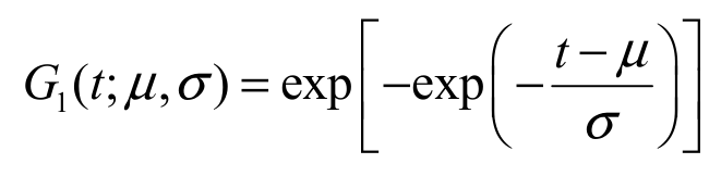 (1)
(1)for t IR, m IR and >0. In a recent paper, Cordeiro et al. (2013) proposed a generalization for the Gumbel model using the so-called exponentiated generalized (EG) class of distributions defined by the cdf expressed as Equation 2:
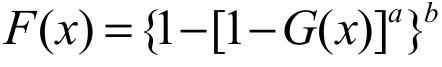 (2)
(2)where > 0 and b > 0.
The probability density function (pdf) corresponding to Equation 2 is given by Equation 3:
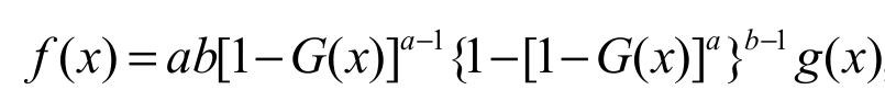 (3)
(3)where g(x) = dG(x)/dx is the baseline pdf. Thus,
Cordeiro et al. (2013) studied the so-called exponentiated generalized Gumbel (EGGu, for short) distribution by inserting Equation 1 into Equation
2. Later, Andrade
et al. (2015) investigated in
detail several mathematical properties for the EGGu
model. In this paper, we will follow the methodology used by Cordeiro et al.
(2013) and Andrade
et al. (2015), but we will consider
a standardized version of the Gumbel distribution, the so-called standardized
Gumbel (SGu) model. Let T be a random variable having cdf Equation 1. The SGu
distribution is defined by a linear transformation, 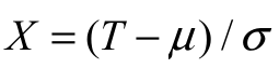 , where
IR
and >0. Without loss of generality, we can
work with the SGu model, since T = +
X, where
IR and >0. The G(x) and pdf g(x) of the SGu
distribution are given by Equation 4 and 5:
, where
IR
and >0. Without loss of generality, we can
work with the SGu model, since T = +
X, where
IR and >0. The G(x) and pdf g(x) of the SGu
distribution are given by Equation 4 and 5:
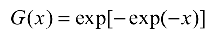 (4)
(4)
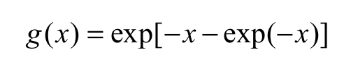 (5)
(5)respectively, for x IR. The goal is to show that our simplified version of the EGGu model has great power of fit to real data and good simulation properties, with the advantage of having only two parameters. Therefore, we define the exponentiated generalized standardized Gumbel (EGSGu) distribution by inserting Equation 4 into Equation 2. The cdf F(x) and pdf f(x) of the EGSGu distribution are given by Equation 6 and 7:
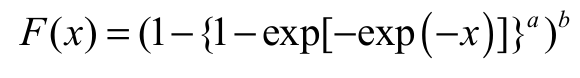 (6)
(6)
 (7)
(7)where > 0 and b > 0. The two extra parameters and in the density Equation 7 can control both tail weights, enabling the generation of flexible distributions, with heavier or lighter tails, as appropriate. There is also an attractive physical interpretation of the model Equation 7 when and are positive integers: Suppose initially that a certain device is composed of components in a parallel system. Consider also that, for each component , there exists a series of subcomponents independent and distributed according to the SGu model. Suppose also that each component b fails if some subcomponent fails. Let Xj1, …, Xja denote the lifetimes of the subcomponents within the j th component, j = 1, …, with common cdf SGu. Let Xj denote the lifetime of the j component and let X denote the lifetime of the device. Hence:
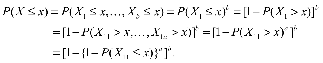 [x]
[x]Thus, the lifetime of the device obeys the EGSGu family of distributions. Besides this introduction, the paper is organized as follows. In the Material and Methods section, we investigated the quantile function and its applications. Next, several mathematical properties of the new model are derived and numerical studies are detailed. In the Results and Discussion section, we used a real dataset to empirically show the power of fit of the EGSGu model and presented the Monte Carlo simulation study.
Material and methods
Quantile function
As an additional characterization of X, we define in this section the quantile function (qf) of the EGSGu model. This function comes directly from the inversion of the cdf Equation 6. Thus, the qf of X is given by Equation 8:
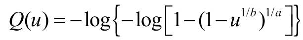 (8)
(8)where u (0,1). There are many important practical applications for Equation 8. For example, occurrences of the random variable X can be easily obtained from a uniform random variable U by X = Q(U). Next, we use Equation 8 to simulate 200 EGSGu (3, 2) occurrences. Figure 1 gives the EGSGu (3, 2) pdf, histogram, exact and empirical cdfs for these simulated data.
In addition, to illustrate the practical utility of Equation 8, it should be mentioned that it can be used to determine the median of X as Med = Q(1/2). Table 1 below presents a small simulation study, whose objective is to compare the empirical medians (Med) generated for different parameter values and random samples of size n = 50, 100, 150, with their corresponding theoretical medians (Med) obtained by Q(1/2). The simulation process is performed in the software R and, to ensure the reproducibility of the experiment, we use the seed for the random number generator: set.seed (103). As expected, the difference between EMed and Med decreases when n increases.
Finally, we present a third application for qf Equation 8, which consists in obtaining in the classical measures of asymmetry and kurtosis of X the Bowley skewness (Kenney & Keeping, 1962) (B) and Moors kurtosis (Moors, 1988) (M). In Figure 2 and 3, we present 3D plots of the M and B measures for selected parameter values, respectively. These plots are obtained using the software ‘Wolfram Mathematica’. Based on these plots, it is possible to conclude that changes in the additional parameters a and b have a considerable impact on the skewness and kurtosis of the EGSGu model, thus corroborating its greater flexibility. Hence, theses plots reinforce the importance of the additional parameters.
Properties of the EGSGu distribution
In this section, we study the structural properties of the EGSGu model.
Linear representations
For an arbitrary baseline cdf G(x), a random variable Yc has the exp-G distribution with power parameter c > 0 say Yc ~ exp-G if its cdf and pdf are given by Hc(x) = G(x)cand hc(x) = cg(x)G(x)c-1 respectively. For a comprehensive discussion about the exponentiated distributions, see a recent paper by Tahir and Nadarajah (2015). Based on some results in Cordeiro and Lemonte (2014), we can express the EG cdf Equation 2 as Equation 9.
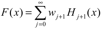 (9)
(9)where 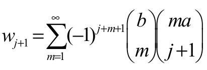 and Hj+1(x) = G(x)j+1
is the exp-G cdf with power parameter j+1. By differentiating Equation 9, we
obtain a similar linear representation for (x) as Equation 10.
and Hj+1(x) = G(x)j+1
is the exp-G cdf with power parameter j+1. By differentiating Equation 9, we
obtain a similar linear representation for (x) as Equation 10.
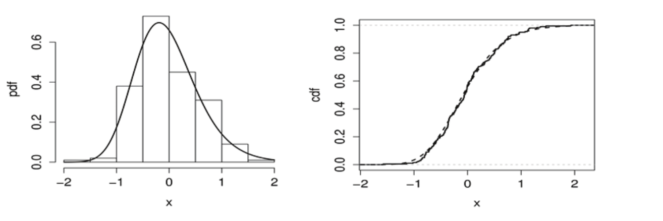
Figure 1.
Plots of the EGSGu (3, 2) pdf, histogram, exact and empirical cdfs for simulated data with n = 200.
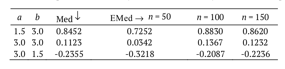
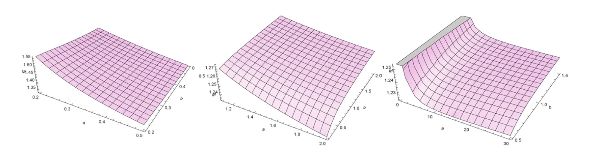
Figure 2.
Plots of the Moors kurtosis for the EGSGu distribution.
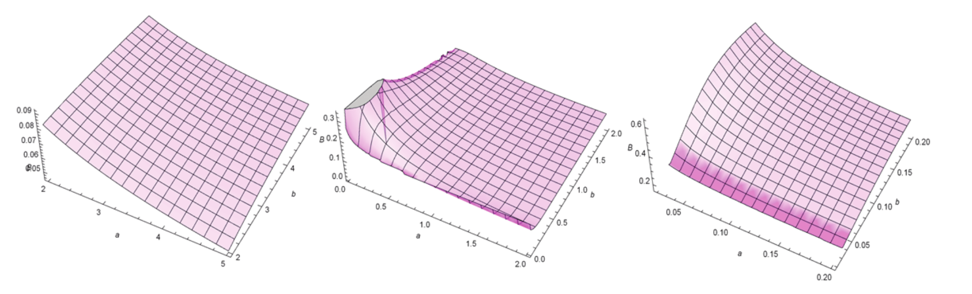
Figure 3.
Plots of the Bowley skewness for the EGSGu distribution.
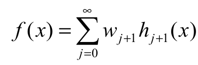 (10)
(10)where hj+1(x) = dHj+1 (x)/ dx. The expSGu pdf with power parameter j+1, hj+1(x), (for j 0) becomes Equation 11:
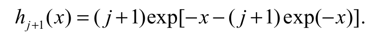 (11)
(11)Combining Equation 10 and 11, we have an important result: The EGSGu density function is a linear combination of expSGu densities. This result can be used to derive some mathematical properties of X.
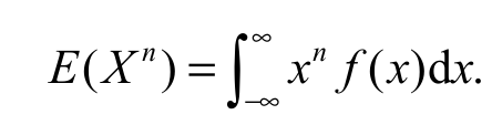
Moments and probability weighted moments
We provide below two ways to compute the n-th moments of X with density Equation 7. Moreover, we go beyond and also present alternative ways to calculate the probability weighted moments, say PWM and denoted by ts,r, for EGSGu model. The first formula for the n-th moments of X become by using Equation 7, follow Equation 12:
 (12)
(12)Alternatively, combining Equation 10 and 11, we can express E(Xn) in terms of expSGu moments. We write Equation 13:
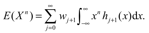 (13)
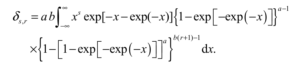
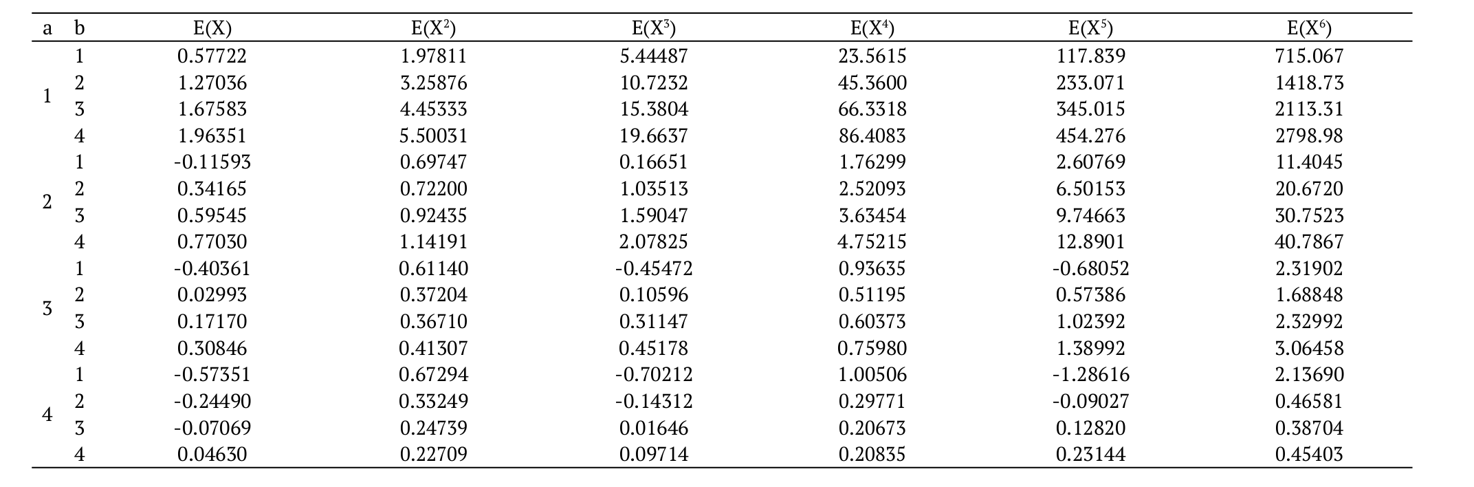
(13)It is very simple to calculate the n-th moment of X computationally, using the expressions Equation 12 and 13. To illustrate it, we provide next a small numerical study, comparing E(Xn) from both formulas. We consider several parameter values and n = 1, 2, 3, 4, 5, 6. The results are shown in Table 2. This table shows that the results agree at five decimal digits of precision for both methods. All computations are obtained using the ‘Wolfram Mathematica’ platform. The (s, r)th PWM of X is defined by s,r = E[Xs (x)r]. Clearly, the ordinary moments follow as s,0 = E (Xs). Next, we derive simple expressions for the PWMs of X defined by Equation 14:
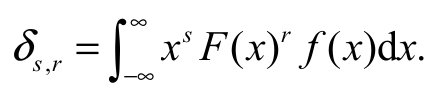 (14)
(14)Inserting Equation 6 and 7 into Equation 14, the PWMs of X can be expressed in a simple form Equation 15:
 (15)
(15)Under simple algebraic manipulation, we can write s,r as Equation 16:
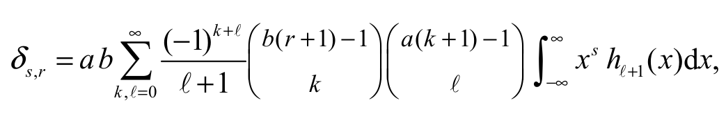 (16)
(16)where hl+1(x) is the expSGu density with parameter (+1). Equation 16 reveals that the PWMs of X can be expressed in terms of the ordinary moments of X ~ expSGu(+1).
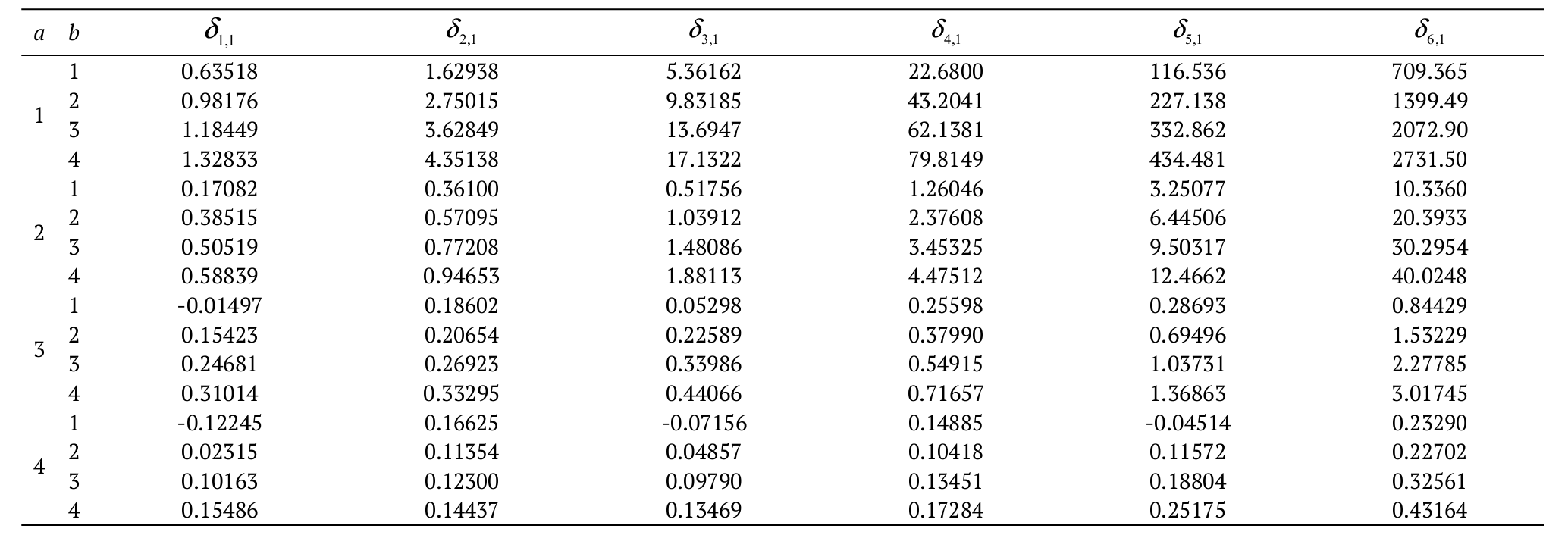
Table 3 gives from Equation 15 the values of s,r for X ~ EGSGu(a, b) and some values of s and r. All computations are performed using the ‘Wolfram Mathematica Software’. Based on the values in Table 3, we conclude that, for fixed r, the PWMs increase when s increases. The opposite happens when we fix parameter s and r increases.
Stochastic comparisons of sample maximum
In this section, we compare the maximum of two independent and heterogeneous samples each following EG class with the same baseline distributions. Let X1:n < X2:n < ... < Xn:n be the order statistics to the random variables X1, X2, …, Xn with X1:n and Xn:n the sample minimum and sample maximum, respectively. The study of Parallel systems plays a prominent role in reliability theory and is equivalent to the study of the largest order statistics. The following two definitions and notation will be needed to prove our main result.
Definition 1: (Shaked
& Shanthikumar, 2007): Let Y and Z be two random variables with,
respectively, absolutely continuous distribution functions M(·) and H(·) densities (·) and (·), and reversed hazard rate functions  and
and  . Hence, Y is said to be smaller than Z in (i) ‘usual stochastic order’,
denoted by
. Hence, Y is said to be smaller than Z in (i) ‘usual stochastic order’,
denoted by  , if
, if  'reversed hazard rate order', denoted by
  .
.
We consider in our main result stochastic comparison in terms of the reversed hazard rate order. Note that reversed hazard rate order implies usual stochastic order. Let In be an n-dimensional Euclidean space with I IR.
Definition 2: (Marshall, Olkin, & Arnold, 2011): Let x = (x1, x2, …, xn) and y = (y1, y2, …, yn) be two vectors in In. The vector x is said:
(i) to majorize the vector y  if
if 
 ;
;
(ii) to weakly supermajorize the vector y (say, ) if
) if 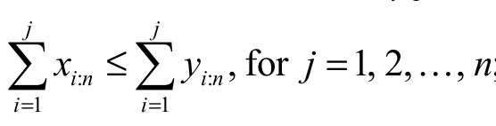 ;
;
(iii) to weakly submajorize the vector y (say,  ) if
) if 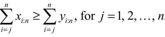
Notation: Let us include the following notations.
(i)
(ii)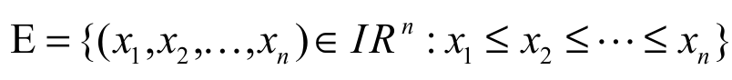
(iii)
(iv)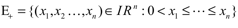
Consider X a random
variable with continuous distribution function G(x) and pdf g(x). For I = 1, 2, …, n, consider
also Xi ~ EG(ai,
bi, G) and Yi ~ EG(ci,
di, G) two sets of n independent random variables where the baseline G(x)
is homogenous and common to both sets of random variables. Suppose that Fn:n(.)
and Hn:n(.)
are the cdfs of Xn:n and Yn:n, respectively.
Hence,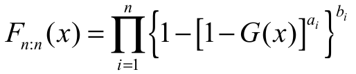 and
and 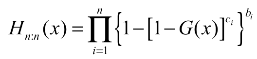 .
.
We can also notice that if  and
and are, respectively, reversed hazard rate functions of Xn:n and Yn:n, then
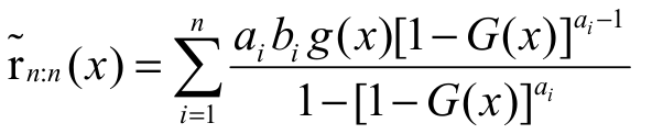 and
and 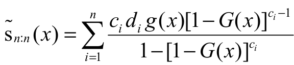 .
.
The following lemmas will be needed to prove our main result.
Lemma 1 (Marshall et al., 2011, p. 86): Let :IIR. Then, (a1, a2, …, an) (b1, b2, …, bn) implies (a1, a2, …, an) (b1, b2, …, bn) if, and only if, is decreasing and Schur-convex on In.
Lemma 2 (Kundu, Chowdhury, Nanda, & Hazra, 2016): Let 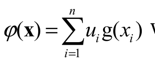 with x D and let I
IR
be an interval. Consider a function g:I
IR. If u=(u1, u2, …, un) E+ and g(.) is
decreasing and convex then (x)
is Schur-convex on D.
with x D and let I
IR
be an interval. Consider a function g:I
IR. If u=(u1, u2, …, un) E+ and g(.) is
decreasing and convex then (x)
is Schur-convex on D.
Consider the following vectors belonging to In: a = (a1, a2, …, an), b = (b1, b2, …, bn), and c = (c1, c2, …, cn).
Theorem (Main result of the section): Suppose Xi ~ EG(ai,
bi, G) and Yi ~ EG(ci,
di, G) with Xi
and Yi two sets of
mutually independent random variables and I
= 1, 2, …, n. Also suppose that a,c D+ and b E+
Then,  implies Xn:n
rhrYn:n.
implies Xn:n
rhrYn:n.
Proof. Let  Differentiating
 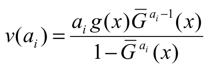 partially with respect to ai, we have
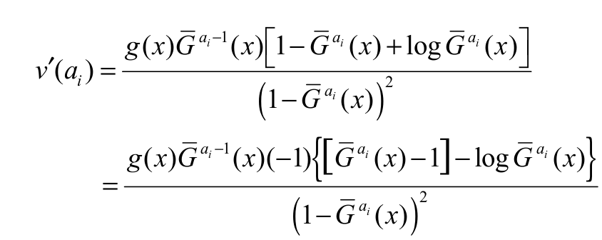 [proof]
 We note that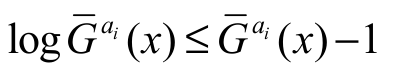 since log x x - 1 for all x > 0. Hence,(ai) 0 and v(ai) is decreasing in ai. By differentiating again v’(ai) with respect to ai, we obtain
 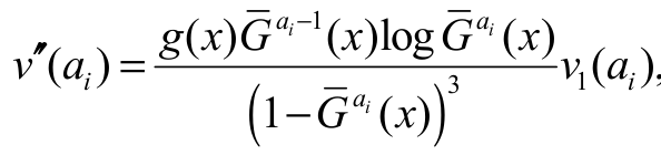 with
with 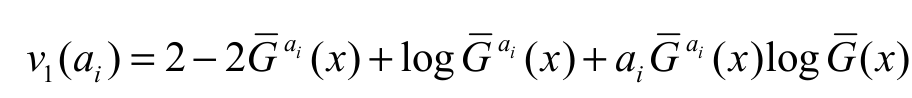 . Taking the derivative of v1(ai) with respect to ai, we obtain
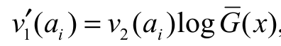 where
where  . Finally, by differentiating v2(ai), also with respect to ai, we have
 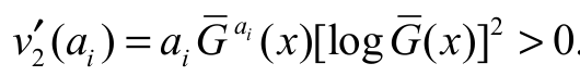 .
.
It is easy to see, for ai
> 0, the following chain of implications, decreasing in ai
  convex in ai.
Thus, by Lemma 1 and Lemma 2, the proof is obvious.
Considering that the theorem holds for any continuous baseline G we naturally have the following corollary.
Corollary (Result applied to EGSGu
distribution): Suppose Xi ~ EGSGu(ai, bi) and Yi ~ EGSGu(ci, bi) with Xi and Yi two sets of mutually independent random variables and
i = 1, 2, …, n. Also suppose that a,c D+
and b E+
and Then,  implies Xn:n
rhrYn:n.
implies Xn:n
rhrYn:n.
Dual generalized order statistics
The dual generalized order statistics (dgos) were introduced in Burkschat, Cramer, and Kamps (2003) as a model for descending ordered random variables and admits as special cases reversed ordered order statistics, lower k-records and lower Pfeifer records (Arnold, Balakrishnan, & Nagaraja, 1998). In this section, we present general expressions for dgos from the EG class. Next, we present results for the EGSGu distribution. We derive an explicit expression for the density of the mth (1 m n) dual generalized order statistic X* (m, n, v, k), say fx*(m,n,v,k) (x), in a random sample of size n from the EG class. By definition we have Equation 17:
 (17)
(17)where 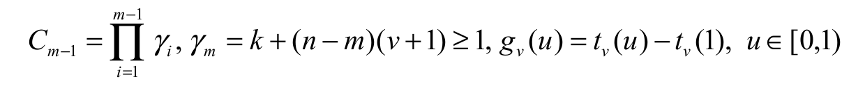 and
and  , v
IR. According to Equation 17, we can rewrite it in two cases, follow Equation 18:
, v
IR. According to Equation 17, we can rewrite it in two cases, follow Equation 18:
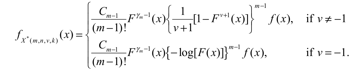 (18)
(18)Case I: For v - 1
Using the binomial expansion in the first sentence of Equation 18 and inserting cdf Equation 2 and pdf Equation 3, we readily obtain Equation 19:
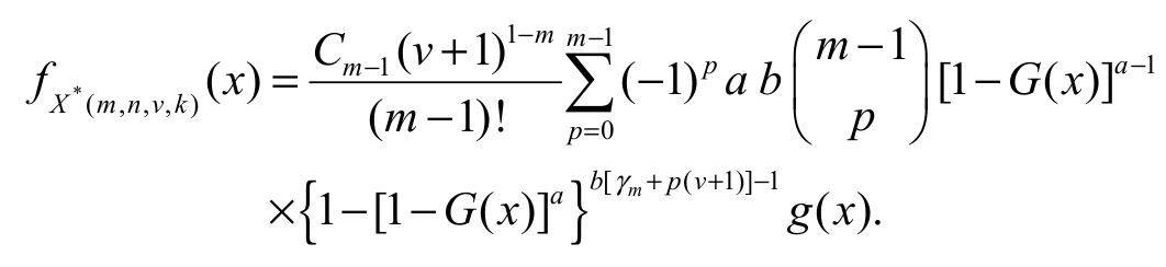 (19)
(19)For any real non-integer (|z|<1), Equation 20:
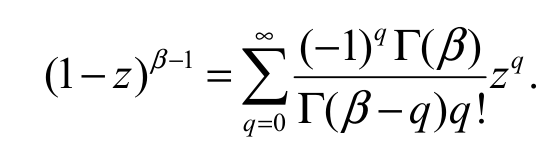 (20)
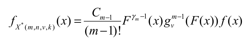
(20)By applying the last equation twice in Equation 19 and after simple algebraic manipulation, we write fx*(m,n,v,k) (x) as Equation 21:
 (21)
(21)where 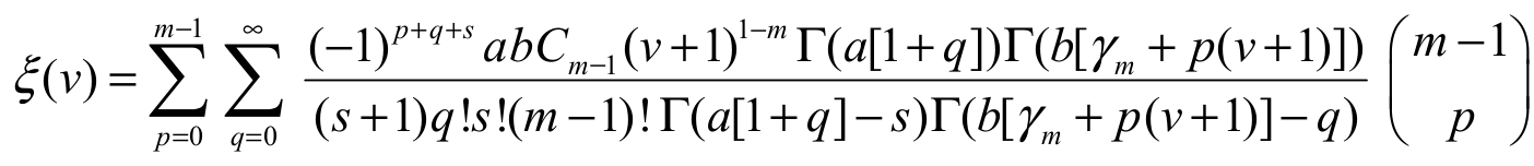
Case II: For v = -1.
By expanding the logarithm function in power series and then using an equation for a power series raised to a positive integer given in Gradshteyn and Ryzhik (2007) (Section 0.314), we have Equation 22,
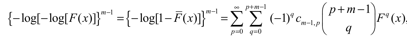 (22)
(22)where and the coefficients cm-1,p(for p = 1, 2, …) are determined from the recurrence equation
 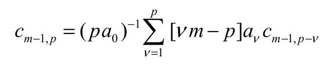 with cm-1,0 = a0m-1. From Equation 22, the second sentence of
Equation 18 reduces to
with cm-1,0 = a0m-1. From Equation 22, the second sentence of
Equation 18 reduces to 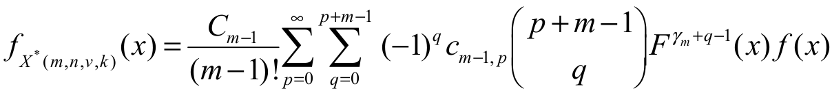
Analogously, inserting Equation 2 and 3 in the previous equation and applying Equation 20 twice, the pdf can be expressed as Equation 23,
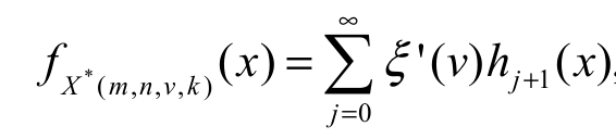 (23)
(23)where 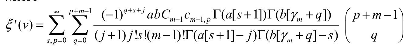
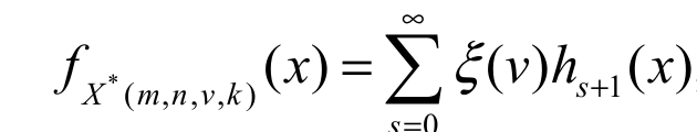
Hence, cases I (Equation 21) and II (Equation 23) can be summarized as (for baseline G distribution) Equation 24:
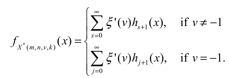 (24)
(24)Based on the previous equation, we can easily obtain the dgos of EGSGu distribution since it depends on exp-G densities. Furthermore, several mathematical quantities of the EG dgos can be obtained from those quantities of exp-G distributions. We provide an example for the dgos moments from EGSGu distribution. Before that, an additional comment on the moments of the expSGu is in order. Inspired by Andrade et al. (2015), we can find a formula for the tth moment Zc ~expSGu of with power parameter c > 0. By setting w = exp{-z}, and using Andrade et al. (2015)'s Equation 14, the tth moment of Zc ~expSGu can be written as Equation 25:
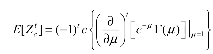 (25)
(25)Thus, the tth moment dgos of the EGSGu distribution can be expressed from Equation 24 and 25 as:
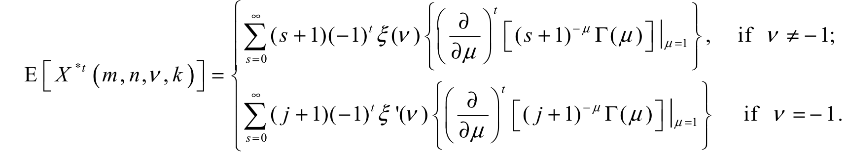 [EGSGU]
It is well known that if v = 0, k = 1 then X* (m, n, v, k) reduces to the (n-m+1)th order statistics Xn-m+1 : n from the sample X1, …, Xn, and when v = -1, then X* (m, n, v, k) reduces to the mth lower k-record value. The main result of this section is given by Equation 24.
Results and discussion
Real data illustration
We
adjusted the EGSGu model given in Equation 7, which contains
just two parameters, and compared the results with other important models in
the literature. We considered the EGSGu distribution
and two Gumbel Lehmann's alternatives sub-models, denoted by EISGu and EIISGu, respectively.
In addition, we have adjusted the models proposed by Mahmoudi
(2011) (BGP distribution), Nadarajah and Eljabri
(2013) (KwGP distribution), and Silva, Ortega, and
Cordeiro (2010) (BMW distribution). Their respective densities are given by  , and
, and  ,
,
where 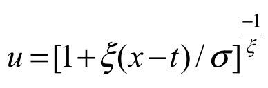 and
and  is the beta function.
The data set was obtained from Murthy, Xie, and Jiang (2004), and consists of the times between failures for repairable items. In Table 4 we provide the MLEs (and their standard errors in parentheses) for all fitted models.
Table 4 also lists the values of the Akaike information criterion (AIC), Bayesian information criterion (BIC) and corrected Akaike information criterion (Caic) statistics. In general, it is considered that lower values of these criteria indicate better fit to the data. With the exception of the Caic of the EISGu model, the figures in Table 4 reveal that the EGSGu model has the lowest AIC, BIC and Caic values among all fitted models. Thus, the proposed EGSGu distribution is the best model to explain these data. Plots of the estimated pdf and cdf of the EGSGu distribution and the histogram of the data are displayed in Figure 4. These plots clearly reveal that the EGSGu model fits the data adequately and then it can be chosen for modeling these data.
Simulated data illustration
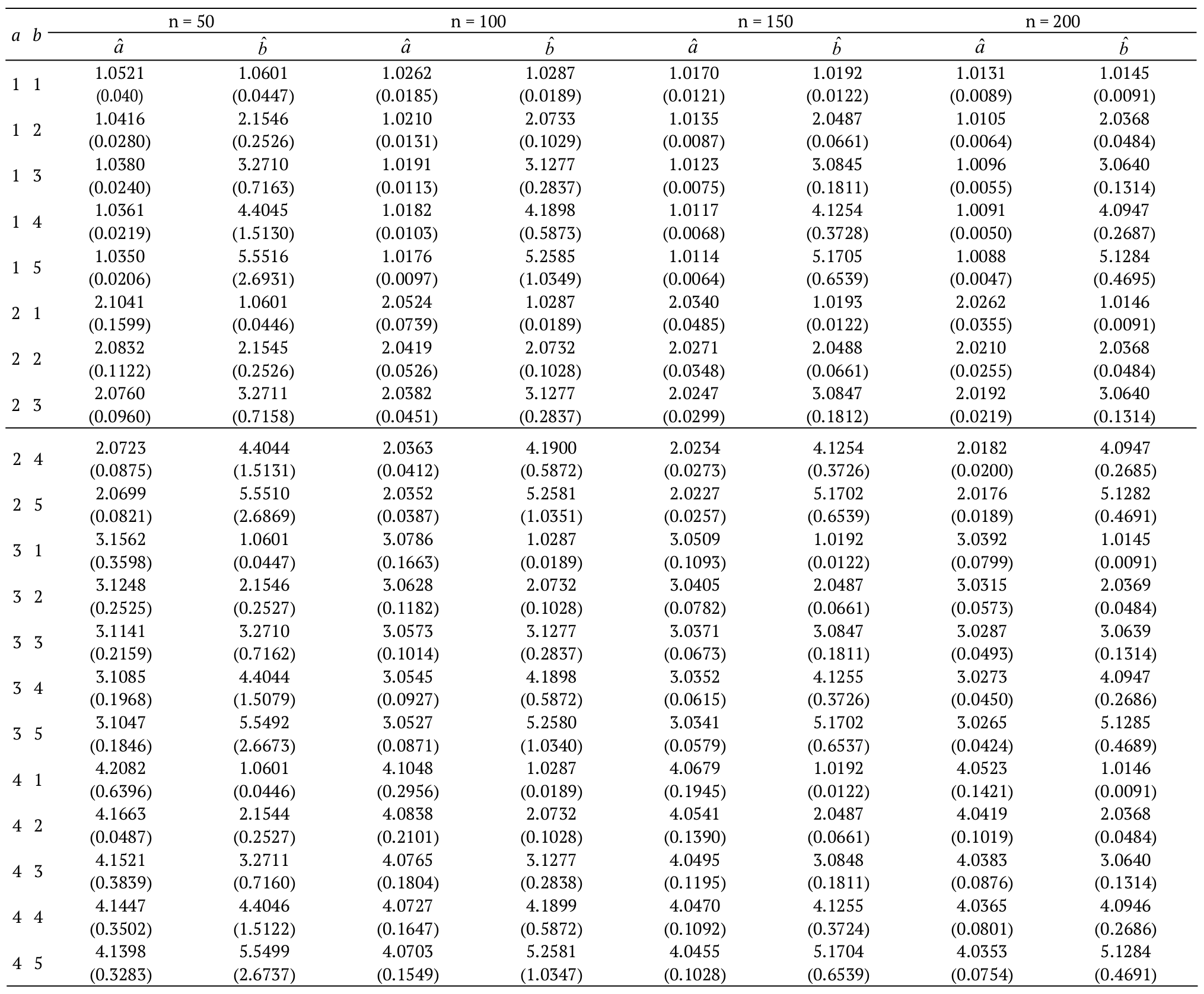
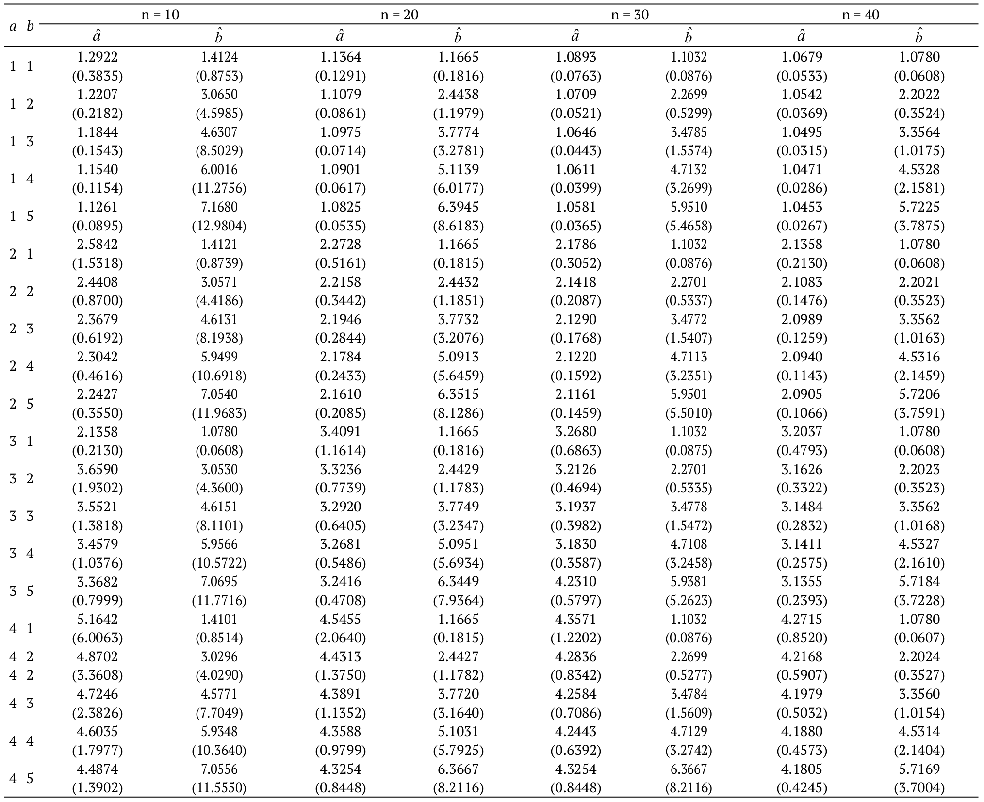
We investigated, by means of a simulation study, the behavior of the MLEs for the parameters of the EGSGu model by generating from qf Equation 8 with samples sizes n = 50, 100, 150, 200 and selected values for a and b. The simulation process is based on 10,000 Monte Carlo replications, performed in the software R using the simulated-annealing (SANN) maximization method in the maxLik script. The results of these new simulations are presented in Table 5 and 6, which contain the estimates and their estimated asymptotic variances in parentheses. These results reveal that, for all estimates, in general, the biases and variances decrease as the sample size increases.
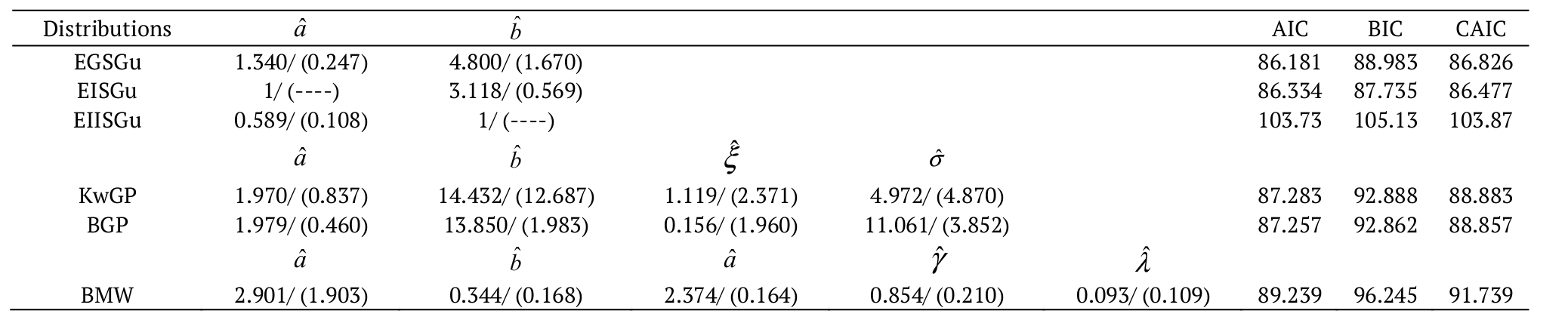
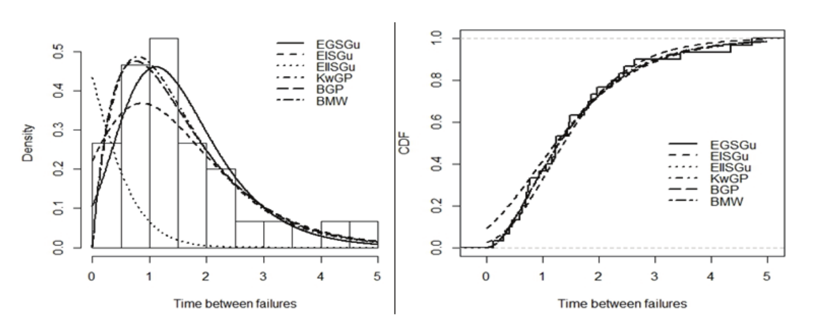
Figure 4.
Estimated pdf and cdf of the EGSGu model for the times between failures for repairable items.
Conclusion
In this article, we propose and study a new two-parameter distribution with real support called the exponentiated generalized standardized Gumbel distribution (EGSGu). Our proposal includes both Lehmann’s type I and II transformations as special cases. We study some mathematical properties of the new model. The model’s parameters are estimated by the maximum likelihood method. A simulation study reveals that the estimators have desirable properties. We empirically prove that the new distribution provides a better fit to a real dataset than other competitive models.
Acknowledgements
We thank two anonymous referees and the associate editor for their valuable suggestions, which certainly contributed to the improvement of this paper. Additionally, Thiago A. N. de Andrade is grateful for the financial support from Capes (Coordenação de Aperfeiçoamento de Pessoal de Nível Superior).
References
Andrade, T. A. N., Rodrigues, H., Bourguignon, M., & Cordeiro, G. M. (2015). The exponentiated generalized Gumbel distribution. Revista Colombiana de Estadística, 38(1), 123-143. doi: 10.15446/rce.v38n1.48806
Arnold, B. C., Balakrishnan, N., & Nagaraja, H. N. (1998). Records. New York, NY: John Wiley Sons.
Burkschat, M., Cramer, E., & Kamps, U. (2003). Dual generalized order statistics. Metron, 61(1), 13-26.
Cordeiro, G. M., & Lemonte, A. J. (2014). The exponentiated generalized Birnbaum–Saunders distribution. Applied Mathematics and Computation, 247, 762-779. doi: 10.1016/j.amc.2014.09.054
Cordeiro, G. M., Ortega, E. M. M., & Cunha, D. C. (2013). The exponentiated generalized class of distributions. Journal of Data Science, 11(1), 1-27.
Gradshteyn, I. S., & Ryzhik, I. M. (2007). Table of integrals, series, and products. Troy, NY: Academic press.
Kenney, J. F., & Keeping, E. S. (1962). Mathematics of statistics. Part 1 (3rd ed.). New York, NY: D. Van Nostrand Company, Inc.
Kundu, A., Chowdhury, S., Nanda, A. K., & Hazra, N. K. (2016). Some results on majorization and their applications. Journal of Computational and Applied Mathematics, 301, 161-177. doi: 10.1016/j.cam.2016.01.015
Mahmoudi, E. (2011). The beta generalized Pareto distribution with application to lifetime data. Mathematics and Computers in Simulation, 81(11), 2414-2430. doi: 10.1016/j.matcom.2011.03.006
Marshall, A. W., Olkin, I., & Arnold, B. C. (2011). Inequalities: theory of majorization and its applications. New York, NY: Springer.
Moors, J. J. (1988). A quantile alternative for kurtosis. Journal of the Royal Statistical Society. Series D, 37(1), 25-32. doi: 10.2307/2348376
Murthy, D., Xie, M., & Jiang, R. (2004). Weibull models. Wiley series in probability and statistics. New Jersey, NJ: John Wiley and Sons.
Nadarajah, S. (2006). The exponentiated Gumbel distribution with climate application. Environmetrics, 17(1), 13-23. doi: 10.1002/env.739
Nadarajah, S., & Eljabri, S. (2013). The Kumaraswamy gp distribution. Journal of Data Science, 11(4), 739-766.
Shaked, M., & Shanthikumar, G. (2007). Stochastic orders. New York, NY: Springer.
Silva, O. G., Ortega, E. M. M., & Cordeiro, G. (2010). The beta modified Weibull distribution. Lifetime Data Anal, 16(3), 409-430. doi: 10.1007/s10985-010-9161-1
Tahir, M. H., & Nadarajah, S. (2015). Parameter induction in continuous univariate distributions: Well-established G families. Anais da Academia Brasileira de Ciências, 87(2), 539-568. doi: 10.1590/0001-3765201520140299
Author notes
franksinatrags@gmail.com