Statistics
The use of control chart for a continuous monitoring of the water-oil ratio in fields of the Potiguar basin/Brazil
The use of control chart for a continuous monitoring of the water-oil ratio in fields of the Potiguar basin/Brazil
Acta Scientiarum. Technology, vol. 42, 2020
Universidade Estadual de Maringá

This work is licensed under Creative Commons Attribution 4.0 International.
Received: 19 March 2018
Accepted: 10 July 2018
Abstract: Nowadays, petroleum is the most used energy source in the world, however it also produces a great volume of a residue denominated produced water (PW). This water has no commercial value and requires treatment, due to potential contaminants in its composition, in order to be destined for disposal or reinjection during recovery methods. In this way, the produced water management needs specific process support it, becoming costly. Therefore, the present work proposes a continuous monitoring methodology of the water-oil ratio, aiming to subsidize the field viability analyses. Once that the water-oil ratio data are auto-correlated, some adjustments are needed before the application of the control charts. Therefore, ARIMA models were adjusted to the data, evaluating the accuracy of the models, then, the control charts were built based on the residues. In this paper, the type of control charts considered was a Shewhart for the averages. The performance of the chart was evaluated through simulations and it was determined that it is efficient to detect big deviations, but slow to small deviations.
Keywords: water-oil ratio, produced water, shewhart control chart, ARIMA model.
Introduction
Oil is currently the most used energy source in the world. However, its extraction produces a considerable volume of water, known as connate water or produced water.
The origin of this water is associated with the rock formation, being always present in the reservoirs. However, in order to displace it, its saturation needs to exceed a minimum value. So, when the mobility of water overcomes the oil, the water-oil ratio (WOR) increases. It is calculated according to the volume of produced water in relation to the volume of oil.
In field operations, the oil, water and gas are separated in the reservoir, however they are not produced separately because when these fluids flow through the production pipes, they are subjected to agitation and shear stress, forming emulsified phases. Thus, requiring separation processes (primary processing) as well as specific treatments in order to reuse (Reinjection) or discard the produced water.
It is important to highlight that the economic interest focused in the oil production and the produced water (PW) does not have any commercial value. In addition, the PW carries a large amount of impurities and pollutants (chemical additives, organic and inorganic compounds, salt, oil and radioactive materials). The process of separation can be simple or complex, depending on the fluid characteristics, location of the reservoir and economic interests.
In addition, the PW is the largest waste produced during the production of oil and gas. In a world scale, the volume of PW exceeds their production. In this way, the processes of the management and treatment of this water result in high costs, associated with the high volumes, complexity of the treatment processes and reuse.
Thomas (2001) highlighted that in the world, on average, the production of a 1 m3 day-1 of oil produces 3 to 4 m3 of PW. Fakhru’l-Razi et al. (2009) supported this statement and added that the world production of PW when compared to oil is 3 to 1.
In this way, the management of produced water is an inherent problem associated with the process of oil production. Veil (2007) stated that, as any other residue, the produced water incurs costs and needs to be managed, in addition for being the largest production residue. Therefore, this author suggests a three level prevention hierarchy:
1. Use technology to minimize the production of water;
2. Reuse and recycle;
3. If none of these levels are practical, the elimination is the last option.
In addition, Clark and Veil (2009) affirmed that the management costs of such high volume of residual water is a key issue for the oil and gas producers, affecting directly the decision to produce certain fields.
Thus, the continuous monitoring of this ratio provides subsidies to manage the viability of the reservoirs, providing data regarding the potential environmental damage that may happen if a large volume of PW is produced. The use of monitoring tools is critical to the management of the production fields.
In General, in production processes, the monitoring of certain measures aid the management team to discover deviations in control levels of the process that generate extra costs. Through such techniques, it is proposed an adjustment of boundaries, helping the team to evaluate the control measures of interest in the process.
According to Montgomery and Runger (2003), the main objective of the control chart is to differentiate the occurrence of special causes, which leads to major changes in the process deviations caused by common or random causes. They were initially proposed by Shewhart (1931) and, traditionally, are composed by three parallel lines: a line that reflects the expected level of operation of the process, and two external lines called upper control limits (UCL) and lower control limit (LCL), calculated according to the standard deviation of any variable or attribute of the process (Shewhart, 1931). It is assumed that a process is in statistical control when all points plotted is in these limits. When a point is outside these limits, it is assumed that it is necessary to intervene in the process, because it is assumed that a special cause occurred out of control state.
The control charts are, therefore, visual tools used for monitoring interest measures. Its importance lies in the fact that, since they are designed correctly, its use is simple. However, they are usually planned and evaluated, assuming that consecutive observations of the process are independent and identically distributed (i.i.d.). Although, this hypothesis is sometimes violated in practice, because some processes may exhibit autocorrelation (Montgomery, 2009).
It is expected that the water-oil ratio data follows a growth trend over time, because the production of oil decreases and the water production increases continuously, having a trend and show autocorrelation. Therefore, because this autocorrelation is inherent to the data cluster, it must be taken into account during the planning of control charts. This avoids incorrect estimates of its parameters, reduce the rate of false alarms and the number of samples needed to detect offsets in the average of the process ( Wiel, 1996; Reynolds & Lu, 1997; Vanbrackle III & Reynolds, 1997).
Several papers highlight that, in cases of autocorrelated data, it is possible to adjust an estimation model of the observations and perform a process monitoring with control charts for the resulted i.i.d. residues (Montgomery & Mastrangelo, 1991; Superville & Adams, 1994; Zhang, 1997; English, Lee, Martin, & Tilmon, 2000;Koehler, Marks, & O'Connell, 2001; Testik, 2004).
It is important to highlight that the study of monitoring models for random variables, including those with autocorrelation, is extensive and consolidated, however, studies of models for monitoring the ratio of two random variables are relatively recent. In addition, there are no records of papers that used control charts of autocorrelated data to monitor this variable of the oil industry. Celano and Castagliola (2015) proposed a model to monitor the production processes in which the proportion of two materials in the composition of a product must be kept under control, whereas variables with normal distribution. However, Tran, Castagliola, and Celano (2016) proposed the use of unilateral CUSUM chart to monitor the ratio of two variables with bivariate normal distribution.
Therefore, the objective of this paper was to propose a method for monitoring WOR in oil fields located at the Potiguar Basin. The Control Charts (Shewhart) were applied to the residues of the ARIMA model obtained for each field studied, in order to provide subsidies for better management of the produced water and economic viability of these fields. This approach was applied once that a lack of control was detected, so, the interpretation is that the proportion of produced water in relation to the oil production turn that field unfeasible.
According to Gujarati and Porter (2006), ARIMA models analyze the stochastic or probabilistic properties of time series, being represented by ARIMA (p, d, q), where p is the number of autoregressive terms of the model; d, the number of times necessary to differentiate the series before it becomes stationary; and q, the number of terms for moving averages, being p, d and q integers greater than or equal to zero.
So the application and adjustment of an ARIMA model that is appropriate to the data, has the focus to remove autocorrelation, obtaining the independent residues and applying control charts to these, so the monitor the process with the conventional techniques of SPC (Statistical Process Control) can be used.
Material and methods
The methodology proposed for monitoring the water-oil ratio is based on the analysis of the monthly water and oil production data of fields located at the Potiguar basin between 2006 and 2015. The data were obtained through annuals provided by the Agência Nacional do Petróleo, Gás Natural e Biocombustíveis (ANP, 2017) and, after the data collection, it was possible to calculate the monthly water-oil ratio (WOR) values for each field, being this the variable of interest of the model.
Such variable was chosen because it is a measure that makes possible the comparison between the oil fields, regardless their magnitude. In addition, a decision on this measure provides economic subsidies on the viability of the fields.
Historically, the Potiguar Basin is one of largest oil producers in Brazil, however, currently, the oil exploration occurs mainly from mature wells. In theory, mature fields have a larger production of PW when compared with new fields, due to the nature of the exploration process.
In this way, a selection based on the age of the fields was performed for modelling purposes. This restriction was conducted to obtaining a sample with homogeneous characteristics in relation to the variable of interest.
In this step of sample construction, the authors selected fields with more than 15 years of operation and whose data had a behavior that allow modeling, resulting in total of nineteen onshore production fields.
In General, the proposed model can be divided into three main steps, described in Figure 1.
For any ARIMA model adjustment, it is necessary to check the stationarity of the time series. If it does not have this feature, data transformations need to be made until the series becomes stationary. The most common transformations for the ARIMA model are logarithm and the successive differences. At this stage, the software R (R Core Team, 2017) was applied. Successive combinations of the model parameters (p, d, q) were made and the normality of the residuals were tested in the Shapiro-Wilks test. The packets used were the forecast, for the analysis of time series and the placing for the determination of the control limits.
After this step, an ARIMA model is adjusted and its adequacy is evaluated. The residues of the final model will be used in monitoring, being its control limits calculated to achieve a desired performance level. Thus, each of the fields studied was adjusted to a specific model and the normality of the residuals was then tested to validate them.
With the residues of each model set, the control limits for the water-oil ratio for each field were determined.
Predictions for the 2016 data were calculated using the parameters of the adjusted ARIMA model. The residues for 2016 were obtained (through the difference between collected and provided values) and monitored in a control chart in order to assess whether the fields were still under statistical control or not. The term ‘Under statistical control’ means that there was no change in the parameter values (average, for example), validating the monitoring model.
The proposed monitoring methodology can be summarized through the flowchart presented in Figure 2.
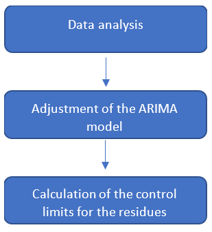
Figure 1.
Overview of the model steps.
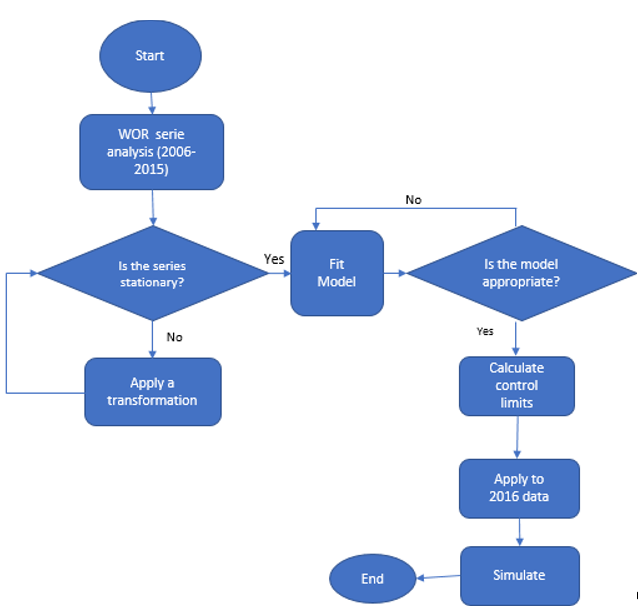
Figure 2.
Proposed metodology flowchart.
A simulation was performed to evaluate the performance of the flowchart regarding the detection ability of deviations for this dataset. The simulation generated 2000 random numbers according to the probability of normal distribution, considering deviations of 10, 50, 100 and 200% in relation to the average values and compared with the previously established control limits. If the value generated was greater than the upper limit or less than the lower limit of control, the process is stopped and the value of samples until this lack of control is filed. This simulation was replicated 5000 times and, from the results, the sample average was obtained until the chart detected the deviation. For simulation purposes, the average number of samples until the signal was set at most 60 (months), obtaining a new set of control limits for this situation.
Results and discussion
After analyzing the time series for the WOR of each field, based on autocorrelation and partial autocorrelation, it was observed that this data does not result in a stationary time series. In this way, the proposed model is based on an estimation of the corresponding ARIMA model for each field, so the residue control charts can be constructed.
To illustrate how the results were obtained, Figure 3 and 4 show the analyzes of Fields I and II (field names cannot be disclosed). They were chosen to illustrate the methodology proposed by dealing with two extreme behaviors during the modeling process. Field I showed a data with simpler modeling behavior and with better results in relation to the normality. In Field II, a more complex model is necessary in order to obtain the adequate residues. In this way, there are two different situations for comparing the results.
It can be observed that the WOR for Field I presents a stationarity tendency, Figure 3. However, it can also be noticed that the autocorrelation (ACF) has a slow decay of direction, suggesting that there is autocorrelation in this data set.
The series resulting from the Field II data follows a different pattern, once that it is observed a tendency to decrease the ratio along time. In addition, the analysis of autocorrelation highlights a very slow decay. Therefore, it is concluded that the series is not stationary.
Those observations were repeated for all the fields selected to compose the sample: the analysis of the WOR ratio data resulted in non-stationary series. Although all WOR data were analyzed in the period from 2006 to 2015 for the studied fields, intermediate periods where the data behaved in a roughly stationary pattern were selected in order to obtain the ARIMA models of these fields.
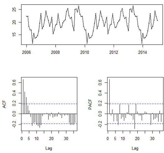
Figure 3.
Graphs of WOR ratio for Field I.
Figure 4.
Graphs of WOR ratio for Field II.
Consequently, the authors first calculated the differences of the original data, considering specific time intervals for each series, and thus a new analysis was performed. Figure 5 and 6 present temporal series of Fields I and II after applying the transformations (and with their functions of autocorrelation and partial autocorrelation).
Therefore, from the analysis of the correlograms, it was possible to observe that, after the calculation of the first difference, the series generated were stationary.
The next steps were the identification and estimation of the parameters (autoregressive and moving average) for the ARIMA model of the selected fields. The criterion used to select the appropriate parameters was based on the analysis of the residues using the Shapiro-Wilks test evaluating if a dataset follows a normal distribution. The p-value measures, in this case, the evidence of the hypothesis that the residue is normal. A p-value above 0.05 confirms the normality of the residuals. Table 1 presents the parameters of the ARIMA model adjusted and P-value of the normality test for the residues.
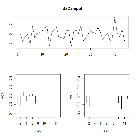
Figure 5.
Graphs of the first difference of WOR data for Field I.
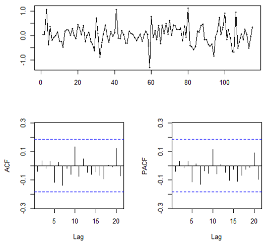
Figure 6.
Graphs of the first difference of WOR data for Field II.
| Field | Adjusted ARIMA Model | P-value |
| I | (1, 0, 0) | 0,8636 |
| II | (3, 2, 4) | 0,1847 |
Once the models were adjusted, the control limits of the graph were calculated for the residues of each one in order to perform a continuous monitoring.
For the elaboration of the control charts, individual observations of the data set analyzed were plotted in order to establish the limits. Once they have been set, the data of the year 2016 was plotted to verify the process control.
To illustrate the methodology adopted and present the preliminary results, the monitoring of Fields I and II will be exposed (Figure 7 and 8).
After determining the graphs, the group carried out a simulation in order to evaluate the performance of the graphics regarding each dataset. Therefore, in order to do that, the maximum sample value was set up to the signal at 60 months, so the graph could detect faster an unmanageability when compared to the traditional graph. This decision was necessary because, since these are monthly data, it didn't make sense an average number until the alarm of 372 months (expected value to the traditional chart with 3 standard deviations). In this way, new control limits were obtained to carry out the simulation.
As a result, it was observed that the control graph for averages shows better performance for large deviations, as can be seen in Table 2.
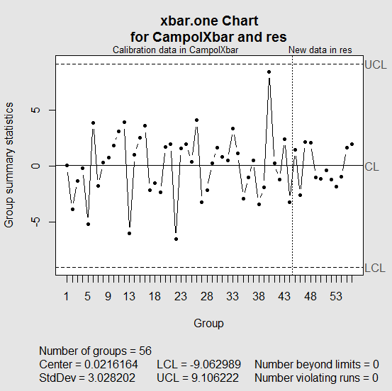
Figure 7.
Control graph for Field I.
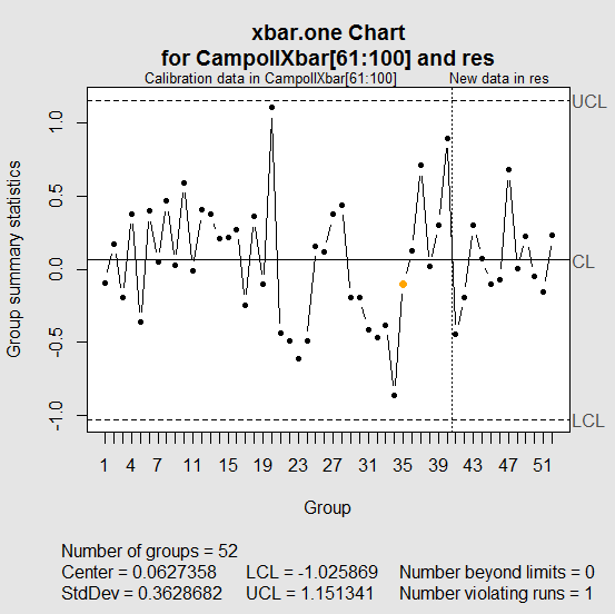
Figure 8.
Control graph for Field II.
| Field | ||||
| 0,1 deviation | 0,5 deviation | 2 deviation | 3 deviation | |
| I | 37,00 | 9,52 | 4,53 | 2,41 |
| II | 47,39 | 10,93 | 4,98 | 2,50 |
Conclusion
Through this study, it was possible to propose a model for the continuous monitoring of water-oil ratio (WOR) and to confirm the natural tendency of continuous increase of this ratio over time. In addition, a significant temporal relationship is perceived for its behavior in which mature wells tend to produce a high level of water.
The proposed methodology presents itself as an important tool for the management of produced water (PW), since it gives subsidies to aid the decision-making in relation to the economic viability of the fields. Since the production of PW only results in costs for the process, due to its no commercial value and needs of previous treatment before being reused or discarded.
Furthermore, it is important to highlight that the data does not follow a pattern in relation to models; each field studied presented a different adjustment model. In this way, it is required to study all fields in order to determine their specific limits.
In general, the average graphs ( ) are efficient to detect quickly large deviations. Also, these graphs are easier to practical use. However, the CUSUM graph is more efficient to detect deviations of lower magnitude.
As a recommendation for future works, there is a need to evaluate the dataset with other control charts, such as multiple-stage boundaries, for example. In addition, it is necessary to evaluate whether the ARIMA model actually meets the modeling of this data.
References
Agência Nacional do Petróleo, Gás Natural e Biocombustíveis [ANP]. (2017). Anuário estatístico da indústria brasileira do petróleo e gás natural. Rio de Janeiro, RJ: ANP.
Celano, G., & Castagliola, P. (2015). A synthetic control chart for monitoring the ratio of two normal variables. Quality and Reliability Engineering, 32(2), 681-696. doi: 10.1002/qre.1783
Clark, C., & Veil, J. (2009). Produced water volumes and management practices in the United States. Condado de DuPage, IL: Argonne National Laboratory Report.
English, J. R., Lee, S.-C., Martin, T. W., & Tilmon, C. (2000). Detecting changes in autoregressive processes with and EWMA charts. IIE Transactions, 32(12), 1103-1113. doi: 10.1080/07408170008967465
Fakhru’l-Razi, A., Pendashteha, A., Abdullaha, L. C., Biaka, D. R. A., Madaenic, S. S., & Abidina, Z. Z. (2009). Review of technologies for oil and gas produced water treatment. Journal of Hazardous Materials, 170(2-3), 530-551. doi: 10.1016/j.jhazmat.2009.05.044
Gujarati, D. N., & Porter, D. C. (2006). Econometria básica (3a ed.). New York: Mc Graw Hill.
Koehler, A. B., Marks, N. B., & O’Connell, R. T. (2001). EWMA control charts for autoregressive processes. Journal of the Operational Research Society, 52(6), 699-707. doi: 10.1057/palgrave.jors.2601140.
Montgomery, D. C. (2009). Introduction to statistical quality control (4th ed.). New York, NY: John Wiley and Sons.
Montgomery, D. C., & Mastrangelo, C. M. (1991). Some statistical process control methods for autocorrelated data. Journal of Quality Technology, 23(3), 179-193. doi: 10.1080/00224065.1991.11979321
Montgomery, D. C., & Runger, G. C. (2013). Applied statistics and probability for engineers (3rd ed.). Hoboken: John Wiley & Son, Inc.
R Core Team. (2017). R: A language and environment for statistical computing. Vienna, AT: R Foundation for Statistical Computing.
Reynolds, M. R. Jr., & Lu, C. W. (1997). Control charts for monitoring processes with autocorrelated data. Nonlinear Analysis, Theory, Methods & Applications, 30(7), 4059-4067. doi: 10.1016/S0362-546X(97)00011-4
Shewhart, W. A. (1931). Economic Quality Control of Manufactured Product. Bell Labs Technical Journal, 9, 364-389. doi: 10.1002/j.1538-7305.1930.tb00373.x
Superville, C. R., & Adams, B. M. (1994). An evaluation of forecast-based quality control schemes. Communications in Statistics-Simulation and Computation, 23(3), 645-661. doi: 10.1080/03610919408813191
Testik, M. C. (2004). Model inadequacy and residual control charts for autocorrelated processes. Quality and Reliability Engineering International, 21(2), 115-130.
Thomas, J. E. (2001). Fundamentos da engenharia de petróleo (2a ed.). Rio de Janeiro, RJ: Interciência.
Tran, K. P., Castagliola, P., & Celano, G. (2016). Monitoring the ratio of population means of a bivariate normal distribution using CUSUM type control charts. Statistical Papers, 59(1), 387-413. doi: 10.1007/s00362-016-0769-4
Vanbrackle III, L. N., & Reynolds, M. R. Jr. (1997). EWMA and CUSUM control charts in the presence of correlation. Communication in Statistics - Simulation and Computation, 26(3), 979-1008. doi: 10.1080/03610919708813421
Veil, J. V. (2007). Research to improve water-use efficiency and conservation: technologies and practice. Condado de DuPage, IL: Argonne National Laboratory Report
Wiel, S. A. V. (1996). Monitoring processes that wander using integrated moving average models. Technometrics, 38(2), 139-151. doi: 10.2307/1270407
Zhang, N. F. (1997). Detection capability of residual control chart for stationary process data. Journal of Applied Statistics, 24(4), 475-492. doi: 10.1080/02664769723657