Mechanical Engineering
Technical analysis of an oven with coupled receiver for scheffler solar concentrator tested under cloudy weather conditions
Technical analysis of an oven with coupled receiver for scheffler solar concentrator tested under cloudy weather conditions
Acta Scientiarum. Technology, vol. 42, e44444, 2020
Universidade Estadual de Maringá

Esta obra está bajo una Licencia Creative Commons Atribución 4.0 Internacional.
Recepción: 04 Septiembre 2018
Aprobación: 17 Julio 2019
Abstract: Most of the solar collectors experiments are carried out under clear-sky conditions to evaluate the maximum performance of collectors, even though this condition is not critical for some uses, such as cooking. The optical and thermal performance of a solar oven heated by Scheffler concentrator is here analyzed in more adverse weather conditions. The receiver for conversion and heat transfer of the concentrated solar energy is coupled to an oven specially developed for this work. The Scheffler concentrator geometry is a lateral cut angled 43.23° of a paraboloid matrix, and it works in a two-axis tracking system, to always maintain its focal image at the stationary receiver with the progression of the Earth rotation and solar declination movements. A model for distributing the daily radiation over the hours is used to compare the results. The time-constant experimental method is considered. The heating and cooling tests were carried out at the official local time. The maximum temperature achieved by the absorber was 328°C, and the maximum average temperature in the oven was 150°C. The results for heat loss factor were evaluated, and the trends for thermal efficiency and optical efficiency factor were analyzed for the system considered.
Keywords: solar energy, scheffler paraboloid concentrator, solar oven, cloudy conditions.
Introduction
Solar concentrators are one of the most promising devices to use solar energy. There are many types of solar concentrators. They can be classified by image formation, i.e., line and point image, and there are subtypes, such as dish concentrator, which produces the second type of the image. However, there are many variations of solar concentrators. One of them is the Scheffler solar concentrator (SSC), a revolutionary contribution from physicist Wolfgang Scheffler.
Its geometry has features that have extended the usage of solar concentrators. Its reflector surface consists in a lateral cut section angled at a = 43.23º from a paraboloid, which makes an elliptical frame. The aperture area is a projection of this elliptical frame over a parabolic guideline, which results in a circle. The focus stays positioned in front of the reflector, at the original place of the parabola focus point. This allows using concentrated solar energy in a shadowed position. The tracking system works in two axes, and the receiver does not move without projecting its shadow on the paraboloidal mirror.
There are some publications that can help manufacture a SSC. A mathematical modeling for an 8 m2 SSC and design generalized chart were presented by Munir, Hensel, and Scheffler (2010) and Reddy, Khan, Alam, and Rashid (2018), respectively. They showed the parameters to take into account when designing the reflector: how to define the parabola equations, structural bars, and how the tracking system works, for example. Both papers recommend developing the design of SSC with reference at the equinox. Furthermore, both authors showed that the aperture area varies with solar declination.
The effects of aperture area variations in the focal image size were studied mathematically by Dib and Fiorelli (2015), and by photogrammetry and Ray Tracing by Ruelas, Pando, Lucero, and Tzab (2014)Ruelas, Palomares, and Pando (2015). Considering a perfect concentrator and perfect tracking system, Dib and Fiorelli found that the variations in aperture area reach the limits of +37% and -38% between both solstices, and when the image is smaller, the aperture area is larger and the concentrated ratio is highest. These results are similar to those in Ruelas et al. (2014).
A comparison between SSC and a traditional dish concentrator was made by Ruelas, Velázquez, and Cerezo (2013). The features of both concentrators were geometrically equivalent. Both receivers were similar and were coupled with a Stirling Engine. For a useful heat of 8423 W, the thermal efficiency of receivers was 0.81 for the dish concentrator and 0.88 for the SSC. According to the authors, the better thermal efficiency of the Scheffler system was a function of the reduction of convection losses due to the difference in the position of receivers.
The mentioned features open new applications for the SSC. For instance, Oelher and Scheffler (1994) built a cooker heated by SSC with a 7 m2 ellipsis area As. The SSC reflected radiations through a window to the receiver pot, the volume of which was about 80 to 100 L. The evaluated power at the cooker was 1.4 kW for 730 W m-2 of beam irradiation incidence.
Patil, Awari, and Singh (2011) analyzed a similar system powered by a SSC of As = 8 m2. The receiver was a pressurized pot of 20 L. The average power and average thermal efficiency of the system was, respectively, 1.3 kW and 0.22 for an average beam solar radiation of 742 W m-2.
Kumar, Prakash and Kaviti (2017) described three systems. The first system is a hybrid autoclave for rural hospitals heated by a SSC and/or natural gas. The SSC reflector As was 10 m2. Steam was generated in an absorber made of an iron block of 230 kg with an internal serpentine. The sterilizing chamber volume was 76 L. The temperature of the sterilizing steam was 121°C. The SSC raised superheated steam to 500°C. For most of the day, the sterilization was observed to occur without support from the natural gas. A second system is a solar crematorium powered by SSC with reflector As of 3.4 m2. The receiver was the cremation chamber covered by a circular metal sheet at concentrator focal plane. Its receiver was built with a hole in the center of this cover to intercept the focal image into the chamber. The system reached 1 kW of power and temperatures greater than 800°C. The third system is for industrial applications of SSC. The authors developed a desalinization system powered by two SSC with 16-m2 As. This system was able to produce 6.5 L of steam per day and per area unit from SSC.
Chandrashekara and Yadav (2017) described an improvement of the receiver applied to another desalination system. A selective material (exfoliated graphite) was tested on absorber surface. This small-scale system was powered by a SSC with 2,7 m2 As. When the SSC is focused on receiver, the coating expands like a sponge structure, and its maximum temperature reaches 643,9°C. The system achieved the maximum thermal efficiency at 0,40 against 0,31 of the absorber without exfoliated graphite.
Indora and Kandpal (2019) reviewed the solar cooking systems powered by SSC. A system installed in a religious temple and manufactured with 106 SSC of As = 10 m2, was able to produce 30,000 daily meals. The systems were mostly equipped with As = 16 m2. One of them is capable to produce 30000 meals per day. These systems were also installed in Indian industries for steam generation.
The application of SSC for a bakery and for a syrup production was reviewed by Panchal et al. (2018). The bakery was heated by SSC with As = 8 m2. Its receiver was a zig-zag absorber inside the oven. An oven temperature of 300°C was measured, with a system thermal efficiency of 0.40 and a 1200 W system power. For the syrup production a kitchen with six SSC with 10-m2 As was built. This system produced 250 L of agave syrup per day.
A point to take into account is that all the publications showed systems evaluated under a clear sky. It is obvious that under rainy or dark cloud conditions, solar concentrators do not produce a focal image, and the system needs to be backed up by another source. Yet, on a light-cloudy day, the concentrated solar energy production is relative to the clarity index. We tested a solar oven under these conditions. A SSC with an aperture area Aap of 2 m2 was built. The SSC receiver was coupled to an oven especially projected for this work. Heating and cooling tests were carried out. A thermodynamic model was made to estimate the energy transferred to the air in the oven. The results of the thermal analysis are presented as follows.
Material and methods
As mentioned before, the SSC was built with Aap of 2 m2 at the equinox, equivalent to an As of 2.76 m2, with a pendulum clockwork tracking system. The SSC was adjusted for the North Pole. The receiver was an absorber plate mounted at the oven back. The temperatures of the outer and inner walls, inner air, and absorber were measured, as well as the meteorological and solar data at the same time. Equation Engineering Solver software (EES) was used for the data analysis.
The concentrator
The SSC was built based on concentrators from the Solare Bruecke community. The structure was mounted with steel bars, and the ellipsis was made of aluminium bars. The reflective surface was made of glass mirror rectangles of 80 x 100 mm. Figure 1 shows a schema of the experimental setup with the SSC, its tracking system and the oven in the focal zone.
The SSC had two tracking systems. One for daily adjustment and the other for seasonal adjustment, which could be represented by a perpendicular axis to this paper sheet, close to the daily axis and parabola profile. The ellipsis has to be flexible to enable the efficient functioning of the seasonal track system, which changes the 𝛼 angle according to the solar declination. Therefore, the SSC changes the parabola profile, changing the aperture area. However, both the focal region and the distance between the receiver and the reflector center point remain constant throughout the year.
The daily tracking system is mounted using steel bars and bicycle parts as a 48-teeth wheel chain drive system, with a rotation axis represented by a dotted line in Figure 1. A counterweight was installed on the rotational base back part of the structure to force the daily rotation of the reflector from the start position (early morning) to the end position (late afternoon). On the front side of this rotational base structure, there is a chain that interacts with the pendulum, controlling the velocity of counterweight action.
The receiver
The receiver is positioned at the back of the oven as indicated in Figure 2. A transparent glass back door covers the absorber, with dimensions of 250 x 250 x 6 mm, which is attached to the oven by screws. The oven absorber is a flat black-painted carbon steel plate. The space close to the front door is the heating functional area. The space near the back door, limited by a removable fence, can be used to carry out other experiments, such as heat storage.
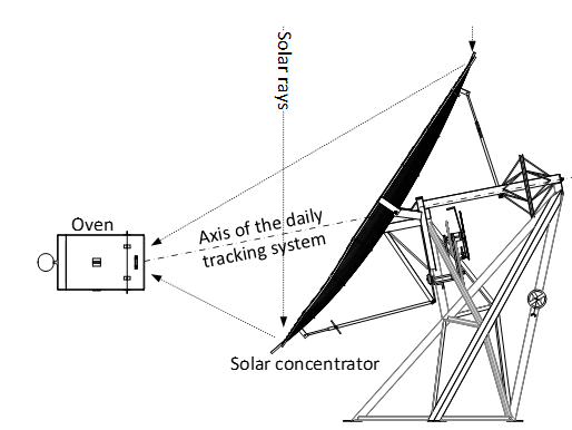
Figure 1 .
Experimental setup schema.
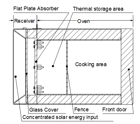
Figure 2.
Cross section view of the receptor-oven assembly.
Figure 3 shows the thermocouples positioning throughout the oven. Temperatures were taken at the inner side of the absorber (T1), inner ambient of the oven (T2, T3, T4 and T5), inner walls (T6, T7, T8 and T9) and external walls (T10, T11, T12 and T13).
Experimental procedure
The measurements of the present work were the oven temperatures, with K-type thermocouple installed in the oven as shown in Figure 3, ambient temperature (T∞) from a local meteorological station (ARACAJU – 83096 Station), and solar irradiation from the Instituto Nacional de Meteorologia (INMET, 2019). The temperature data were registered through the AQX AQ-USB 4350 data acquisition system. To perform a valid experiment, two restrictions recommended by Funk (2000) were adopted: the ambient temperature should be within the range of 20 and 35°C, and the heating test should be carried out between 10 and 14 hours. Then the cooling step was started by defocusing the SSC from the receiver.
Inmet supplied the hourly horizontal global radiation data (IInmet). The Inmet meteorological station was about 1.8 km far from the location of the experimental setup. Hourly horizontal and tilted beam radiation data (Ib; Inmet and Ib; T; Inmet respectively) were obtained from IInmet using correlations adapted from Duffie and Beckman (2013), Equation 1 to 6 presented below. Nonetheless, the distance between Inmet and the experimental location could present some data inconsistencies due to the clouds effects at different times. Therefore, the intensity of the clouds was calculated by the hourly clarity index(kT = IInmet⁄Io). The extraterrestrial solar radiation (Io), was calculated as follows:

where:
Gsc is the solar constant (1367 W m-2 to this work), n is the day of the year, f is the latitude, d is the declination and w2 and w1 are the solar hour, greater and lesser, respectively.
To compare the results with a hypothesis that only daily data would be available, estimations of hourly horizontal beam radiation and hourly tilted beam radiation distributions (Ib; estimated and Ib; T; estimated, respectively) at the experiment location was obtained from the Inmet daily horizontal global radiation data (H) according to the following procedure.
The estimation begins by finding H from the Inmet hourly data (IInmet) summation, and then calculating the daily beam radiation (Hb) and extraterrestrial radiation (Ho). The Hb can be found by correlation with the daily clarity index (KTH = H⁄Ho), as follows Equation 2:
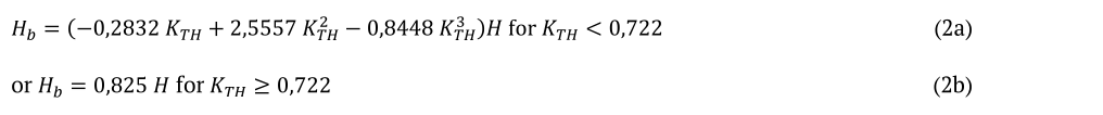
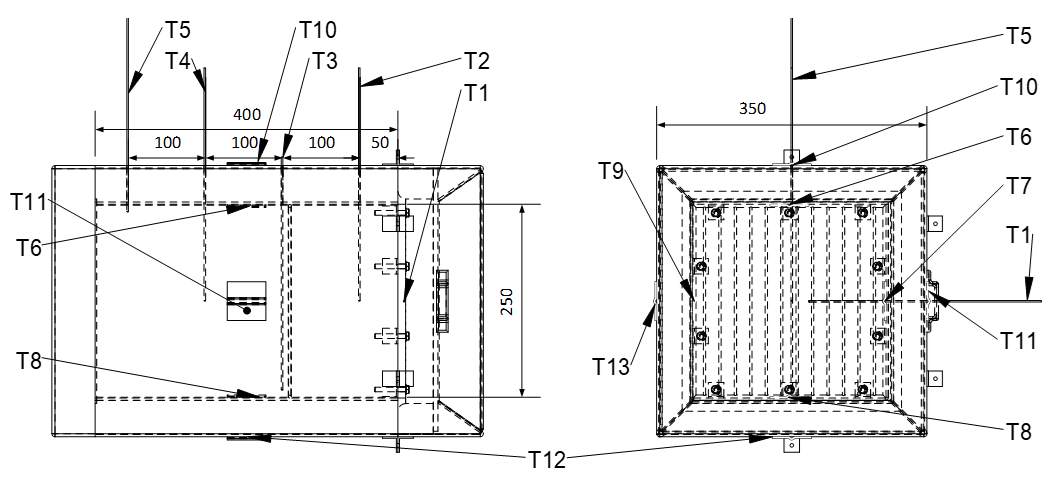
Figure 3.
Thermocouples distribution throughout the oven.
and to calculate the Ho, according Equation 3:

for wss to the sunset angle.
Then, to estimate the hourly global radiation (Iestimated), according Equation 4:

where:
a and b are constants in function of wss and w is an interest hour. Finally, to find the beam radiation for a desired interval of angle hour, according Equation 5:

Equation 5 was also used to calculate the Ib; Inmet by replacing Iestimated with IInmet. The Ib; T; Inmet, the beam radiation orthogonal on the aperture plane per unit of area of the concentrator, was calculated by Rb ratio as shown below, according Equation 6.

The angle between a line to the Sun and an orthogonal line to the aperture area is q = 0º, and the zenith angle is qz.
Thermal analysis procedure
The thermal analysis was developed based on oven temperature data and Equation 7 to 13. Kalogirou (2013) points out that the time constant (T0) as the necessary time to lose a fixed magnitude of heat from the first point of the cooling curve in the form of the difference in temperature between the average temperature in the oven and the ambient temperature (Tav; oven - T∞) to other point was (Tav;oven - T∞)/and, to correspond to the distance of time between both points.
The heat loss factor (F'UL) and optical efficiency factor (F'n0) are calculated by the following equation by the time constant method, as presented by Müllick, Kandpal, and Kumar (1991).
Ar is the receiver area, Aap is the SSC aperture area, Ta and Tb are the Tav; oven, but the first is a time behind the second and the MCp is the product of mass and specific heat capacity of all the oven-receiver elements of Figure 3.
The characteristic curve of the collector can be obtained by the following equation, which is an evaluation of time to the fluid reach Tav; oven = 100ºC in function of beam irradiance (Gb) given by (Tav; oven - T∞)/Gb. If the maximum desired temperature for the analysis of this characteristic curve is to be different from 100, the value of 100 must be replaced with this given Tmax in Equation 9.
The concentration ratio is defined by C = Aap /Ar. The solar beam radiation absorbed by the receiver per square meter of SSC aperture area (S) can be estimated by Equation 10. Figure 4 shows the control volume for this analysis. The incident energy to the oven is represented by SAap.; Ql represents the global thermal losses.
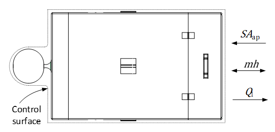
Figure 4.
Control volume considered for thermal analysis.
Since the oven does not have a perfect sealing, the inner pressure is considered to be equal to the atmospheric pressure and might have air leaks during the heating test, air intakes during the cooling test, and during the decrease of the temperatures due the clouds effects. The term mh with an arrow on both sides represents these losses. Subscripts a and b indicate the initial and final states over a 5 min. interval. Thus, equation for S can be estimated by:

In the cooling test, S = 0. The equations to the heat losses, Ql was calculated from:

The product (MCv) is the product of mass and heat capacity of all the parts of the oven, including the inner air volume. Tav; outter wall is the average external walls temperature, and t0 is the time constant. Bi and Fo are Biot and Fourier dimensionless numbers. To calculate mh at air intakes, the average enthalpy between state a and b was considered.

when the temperature at state a is higher than b, the enthalpy was from the surrounding air temperature.

The product of the mass and internal energy of the oven, (Mu) is defined as follows:

In Equation 13, ua and ub are the internal energy of the air at states a and b. The term mCp dT/dt is the product of the mass, specific heat and variation of temperature with the time of component i. The optical efficiency (n0) is the relation of solar radiation incident on the SSC and reflected to the absorber. Irradiation Ib or reflected irradiation, Ibρ, cannot be directly estimated, but if it is multiplied by the product of transmittancet, absorbancea, and intercept factor g , it becomes S. The difference between S and Ibρ is the optical losses of the oven-receiver, quantified by the product (ta). Then S can be written as Equation 14:

The intercept factor (y) includes solar beam radiation spread, mirror imperfections, and track system inaccuracies. The thermal efficiency of the system SSC with oven-receiver can be expressed by heat capacity and mass product of the oven with Tav;oven variation to the all beam radiation on the SSC aperture area, according Equation 15.

Results and discussions
The test was carried out with the solar declination of δ = 11.58 on April 21st (n = 111), when the sunset angle was ωss = 87.72º for the latitude of ϕ = -10.97º. The concentration ratio of the SSC to this day was C = 175. The data were processed with EES (Equation Engineering Solver).
The maximum temperature achieved by the flat absorber was 328°C at 13:05. The maximum temperature achieved inside the oven was 169°C at T2, which was the closest to the absorber and positioned at oven middle height. This can be explained by the influence of the thermal radiation from the absorber. The temperatures difference registered by T3, T4 and T5 in Figure 5 can be explained by the thermocouple positioning shown in Figure 3, and the combination of heat transfer from the flat plate absorber to the inner air and convective effects inside the oven. The average ambient temperature (T∞) was 30.7°C.
Figure 6 allows observing that the temperatures of the inner walls and inner air present a similar profile. The thermocouple from the top wall showed the highest temperature (154°C). Thermocouples T7 and T9, fixed on the west and east walls, showed a maximum temperature of 143°C and 141°C, respectively. This difference may be related to the natural convection in the oven. It would be necessary to install more thermocouples and organize them in a matrix distribution to get 3D temperatures distribution to carry out a better analysis.
Figure 7 shows the temperature profiles for the outer walls. The maximum temperatures recorded by T10, T11 and T12 were 46, 47 and 48°C, respectively. Thermocouple T12, placed on the outer bottom wall, showed the lowest temperature until 12:00 when the ambient temperature decreased slightly, and then, T12 showed a higher temperature than the other thermocouples. This effect can be explained by the smaller space for air circulation under the oven than for other walls.
Figure 8 shows the temperature measurements of the absorber plate, external ambient, average temperatures of the inner ambient and inner and outer walls. It is possible to note the thermal inertia effect by means of the variations shown by the heating curve of the temperatures. These effects were due to the increase or decrease in the clouds quantity and have been observed using the clarity variation in focus imaging as the clouds passed over the solar concentrator, which caused the peaks and valleys in the absorber temperature curve.
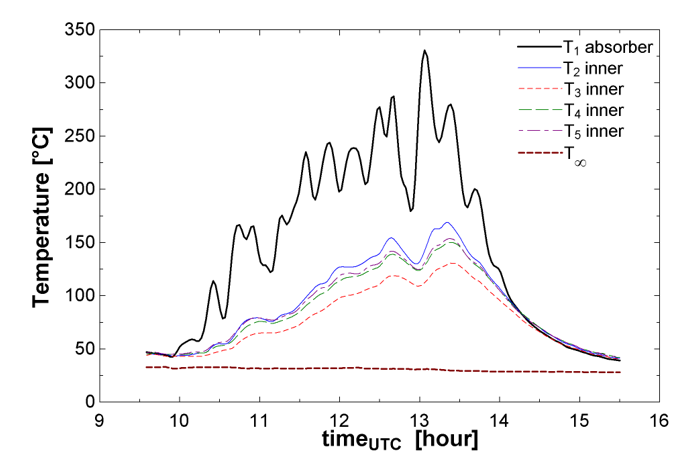
Figure 5.
Temperature measurements of absorber plate, inner and external ambient.
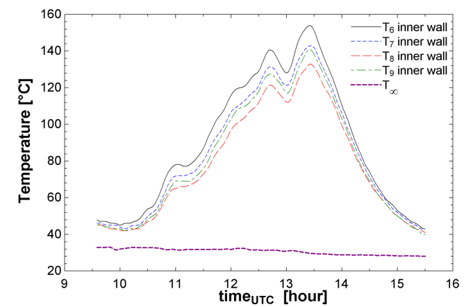
Figure 6.
Temperature measurements of inner walls and external ambient.
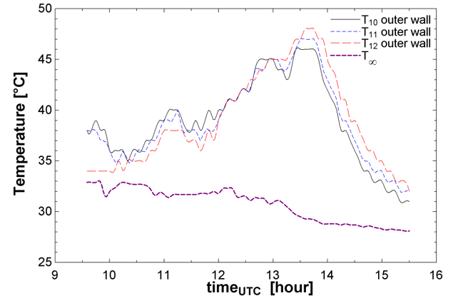
Figure 7.
Temperature measurements of outer walls and external ambient.
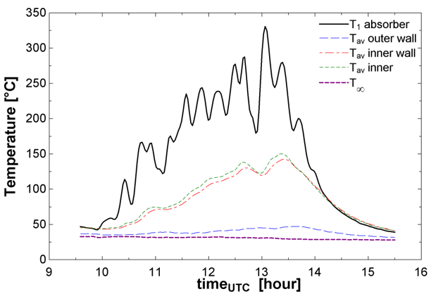
Figure 8.
Temperature measurements of absorber plate, external ambient and averages temperatures of the inner ambient, and inner and outer walls.
An important aspect to point out is that the method to estimate hourly solar radiation brings up some imprecision since it masks the fluctuations due to the clouds. However, it is useful to make a graphic comparison due to the distance between the SSC and the Inmet station.
Figure 9 shows the difference between hourly global radiation from estimating and Inmet data curves. The difference between global (IInmet) and beam radiation (Ib; Inmet) is due to the diffuse radiation. The magnitude variations of this difference in Inmet curves points are due to the presence of clouds over the pyranometer. The same analysis can be used for estimated global (Iestimated) and beam solar radiation (Ib, estimated) curves. Nevertheless, the magnitude of the proportion of diffuse radiation in both Inmet station data curves might give a more accurate quality of solar incidence than the estimated data, which brings the daily overview of the solar radiation. The values of the area integration of hourly global radiation curves were 16075 for the Inmet data and 16200 kJ m-2 for the estimated data. The total global radiation for this day was 163 50 kJ m-2 (Inmet data). These differences are due to the imprecision of Equations 2a and b.
The acquisition of temperatures data was taken in a 5 min. interval, and its curve was more accurate regarding solar energy incidence variations. Then, the average temperature of thermocouples from T2 to T9, Tav; oven and T1 were plotted in Figure 10. The solar beam hourly irradiation data from INMET and estimated were also plotted. Additionally, both solar data were plotted as incidence per square meter on the horizontal (Ib; Inmet and Ib; estimated) and on the SSC aperture plane (Ib; T; Inmet and Ib; T; estimated).
Figure 10 depicts a negative peak in Ib; Inmet and Ib; T; Inmet curves near of 10:30. However, in the T1 curve, this negative peak did not occur. In this curve, there were two different negative peaks between 10:30 and 11:30. There were also two positive peaks in the T1 curve at the same time when the negative peak occurred in the Inmet data. These effects suggest that the clouds were passing over the Inmet sensors and SSC at different times.
Given that is the absorption power per unit of aperture area of SSC, a comparison of all energy losses was also performed, with (Figure 11). is observed to present a similar behavior to (Mu)’ and to the temperature curves of Figures 5 to 8. The increase of intensity of the peaks of agrees with the curve. These significant variations in the curve show the moments when the clouds quantity had increased or decreased, that is, the kT variations.
Temperature T1 was also plotted in Figure 11. This graph shows that the maximum temperature of T1 did not occur at the same time as the maximum and . Probably, it was because of the time of heat transfer in the oven. To calculate , the Biot number varied between 0.0011 and 0.0019, and the Fourier number was 3.97. The losses through mh also were plotted in Figure 11, and it was insignificant, with its maximum at 0.7 W.
The magnitude of may be better understood using the comparison of the temperatures among thermocouples in the oven. If T1 shows quite higher temperatures than the other thermocouples inside the oven, probably most of the incident solar energy converted into heat by the absorber were lost by radiation from the steel plate to the glass cover (see Figure 1). The heat losses may also be occurring by conduction through the oven structure and convection/conduction by the receiver air and the glass cover.
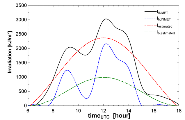
Figure 9.
Inmet data and estimated hourly global radiation (UTC -03:00).
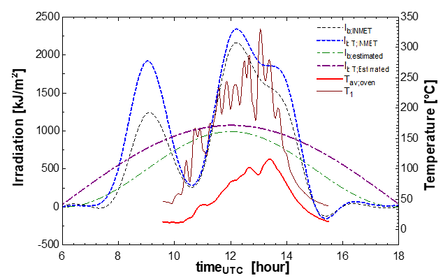
Figure 10.
Plotting of absorber temperature overplotting of hourly beam radiation from estimative and Inmet data, and hourly beam radiation from estimative and Inmet data (UTC -03:00).
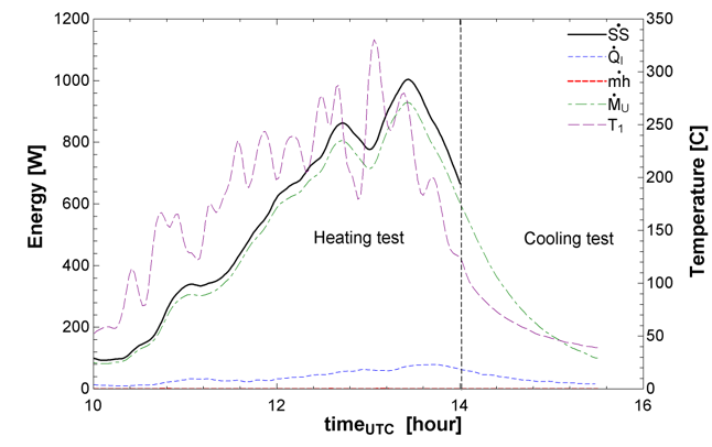
Figure 11.
vs. Ql as a function of UTC.
With the help of Equation 14, the tilted incident beam radiation was calculated. The reflectivity of SSC mirrors, r, was 0.79, the product (ta) was 0.74, and the intercept factor, y, was 1. The average tilted beam irradiance, Gb, was calculated from the data temperature interval of 5 min. Figure 12 shows the curves for Ib; calculated. At maximum, the Gb; calculated was 714 W m-2 over the tilted surface. It is possible to note the similarity with the temperature curves.
Figure 13 shows the curves of the clarity index (kT) and the average oven temperature difference (Tav; oven - T∞) as a function of UTC. The average temperature curve was used to find the time constant (to) of the system. The first point of the to is the initial point of the cooling curve, on the right side of the vertical line in Figure 13. The second point is that equal to (Tav; oven - T∞)/e. In the present work, to was found to be 3888 s. From the value found for to, Equation 7 was used to find a F'UL value of 3.937 W m-2. To calculate the (MCp)’, all the component involved were considered, i.e., thermal insulation, inner air, steel sheet and glass cover were considered.
Note that under clear sky, the first point of to would be at its maximum temperature when the cooling test started. In the temperature curve (Figure 13), the time between the maximum temperature and the start of the cooling test had a small heating and SS > 0. At 14 hours, the SSC was defocused to the receiver and then SS = > 0, as shown in Figure 11.
The kT curve in Figure 13 shows the influence of the atmosphere on incident solar radiation. Such influence occurs mainly by absorptions and reflections back into space of part of the total solar radiation incident in the atmosphere by the water vapor and air (Goswami, Kreith, & Kreider, 2000). In the case herein, it occurs mainly due to the clouds. The greater the cloud intensity, the lesser the kT and Ib; Inmet. Both peaks in the kT curve show the decrease of IInmet. The distance of time between the peaks on kT and temperature curves were due to the distance of the Inmet Station and SSC. The oven temperatures can be considered in agreement with kT variations.
Müllick et al. (1991) consider the maximum temperature as the first point of the cooling curve. In the present work, the first point considered was that from 14:00, when the SSC was defocused from the receiver. This consideration was adopted since the interval between the maximum temperature and the starting of the cooling curve have had a small heating by the concentrator with a decrease of kT (as shown in Figure 13) or increase of the clouds density.
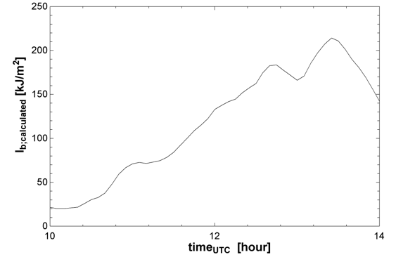
Figure 12.
Curves of beam radiation and beam irradiance on the tilted surface calculated from temperature profiles.
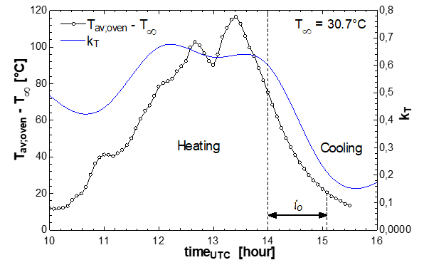
Figure 13.
Average oven-ambient temperature difference as a function of UTC and kT curve.
The analysis of the heating curve of Figure 13 three different time intervals were considered and its results are shown in the steps in Table 1. The analysis consists in calculating the optical efficiency factor and the thermal efficiency, F’ho and hT, respectively. The considerations were studied in seven steps: step 1-overall heating curve; step 2-agreement between oven temperatures and Inmet data (Gb) between 10:00 and 13:25; step 3-between 10:00 and 11:00; step 4-between 11:00 and 12:00; step 5-between 12:00 and 13:00; step 6-between 13:00 and 14:00; step 7-peak 1: between 10:05 and 11:00; step 8-peak 2: between 11:10 and 12:40, and; step 9-peak 3: between 13:00 and 13:25. Figure 9 and 10 show that the correlation of Ib; estimated curves and temperatures are very low.There is no reliability for an F’ho analysis with daily data under cloud conditions. The interval between 10 and 14 hours was made to calculate the overall F’ho and hT of the heating curve. For calculating different time intervals of an hour, the extremes of mainly three temperature rises were considered, i.e., for each peak of temperature (Tb), the previous lowest (Ta) from the same peak was considered, along with its time interval t.
The difference of hT between steps 1 and 2 shows the influence of the clouds on the system thermal performance. By excluding the decrease of temperature as from 13:25, the hT value increased from 7.2 to 14.2%. The high value the F’ho and hT as from the third step, in comparison with the fourth, fifth and sixth steps may be explained by low cloud effects during this period (see T1 in Figure 10 and SS in Figure 11). Yet during the fourth step interval, the cloud effect was the strongest.
For the seventh to the ninth steps, we considered only the interval of time between a negative peak and the next positive peak of average inner temperature (Figure 10), i.e., to consider only the increase of temperatures, which occurred when there was less or no cloud effect. The closeness of interval time of the peak 1 and step 3 resulted in close values of F’ho. At this interval time, the Inmet data shows a decrease of irradiance whereas T1 increases (Figure 10).
Peaks 1 and 3 showed very close values of hT, 0.348 and 0.349. The difference from the F’ho was also small, 0.852 and 0.809, respectively. But these values for peak 2 were lower. The average irradiance, , in time t between Ta and Tb to peak 2 was greater than to peaks 1 and 2. Probably, the variations in F’ho and hT, to the approximate temperature range, derive from the distance between the experimental step up and the Inmet sensor locations. A cloud may have covered the pyranometer without covering the SSC at the same time, as shown by the peaks analysis in Table 1. Sometimes the average temperature curve of the receptor showed a rise when the pyranometer measured a decreasing situation (this is the case of step 9 and part of step 7) as shown by the peaks of the kT curve from Figure 13.
Step 8 was adjusted when both average oven temperature and solar beam radiation curves showed an increase of data values, despite the difference in the time at the peaks of both kT and (Tav; oven - T∞) curves of Figure 13. Figure 14 presents the effect of the difference between Ta and Tb and solar irradiance over F’ho. It is a specific figure of this system for a variation of F’ho, with T∞ = 30.7°C and F’UL; oven = 3.937 W m-2. The figure shows that the greater the Gb, the lesser is the F’ho. For a fixed Gb, the greater the temperature difference, the higher is the F’ho. The slight variation in the slopes of the solar irradiance mark indicates a trend for better efficiency for higher temperature difference than 30°C. Step 1 of Table 1 showed F’ho = 0.334; however, the average values for F’ho in Table 1 is 0.523. By excluding the negative value, the average of hT from Table 1 is 0.189. Figure 14 also indicates that for a Gb close to 350 W m-2, the real F’ho appears around 0.5.
As elucidated by Müllick et al. (1991), Figure 15 shows a similar analytical curve regarding the present work, which presents the required time (in min.) for the air inside the oven to reach Tmax = 100ºC (tT100) as a function of ambient temperature and solar irradiance. This analysis eliminates local influences and allows comparing the SSC of this analysis to the other solar collectors in different locations.
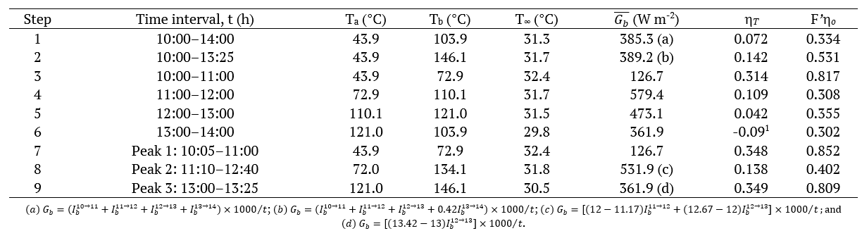
Table 1.
Experimental results for thermal efficiency for Inmet data and optical efficiency factor for Inmet data.
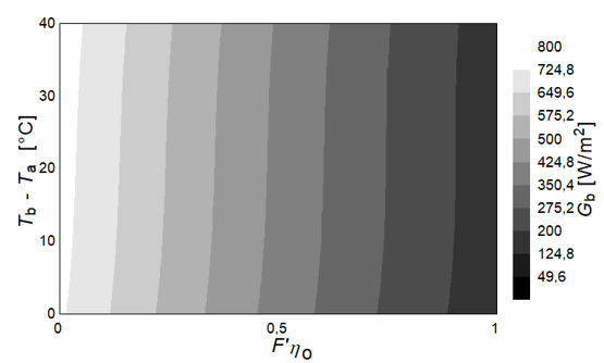
Figure 14.
Influence of (Tb - Ta) and GbT variation on F’ho for T∞ = 30 and F’UL;oven = 3.937 kW m-2.
Figure 15.
Oven characteristic curve.
The usage of solar concentrators under cloudy sky is common for many days along a year. It is thus necessary to carry out a meticulous analysis of the heating curve. On the other hand, the cooling curve analysis is affected by the weather conditions, i.e., wind and ambient temperature.
Conclusion
This paper presents the analysis of an application of SSC with a different oven configuration acting as receiver, and under adverse sky conditions. This oven was designed with similar inner dimensions to standard laboratory ovens and adapted to include the receiver to convert the solar energy into heat.
The results indicate that the thermodynamic model developed to estimate the solar energy transferred by the oven inner air presents fair results since the behavior of the curve SS (Figure 11) is similar to the temperature of the absorber curve. In the same way, the curve of heat losses is in accordance with all the other curves for the thermocouples inside the oven.
Given that the test was carried out under cloudy sky, a meticulous analysis of the oven heating curve is required as shown by the peak analyses in Table 1. The time constant method was helpful to find the overall heat losses factor from the cooling test (F’UL = 3,937 W m-2). The average optical efficiency factor was F’ho = 0.523 and the average thermal efficiency was hT = 0.189. The uncertainties in these values could be reduced by the general graph from Figure 14, which indicates the trends for F’ho. As a suggestion, an additional heater close to the flat plate absorber could be tested to minimize the thermal inertia effect. Nevertheless, the estimated data obtained by the calculations performed herein can be used for carrying out a daily analysis of the solar equipment because the hourly distribution is proportional to the solar hour angle. This experiment showed the possibility for using the solar concentrators also in the unstable weather conditions.
Acknowledgements
The authors are highly grateful to the Fundação de Apoio à Pesquisa e à Inovação Tecnológica do Estado de Sergipe (Fapitec-SE), Tiradentes University (Unit), Laboratório de Catálise, Energia e Materiais do Instituto de Tecnologia e Pesquisa (Lcem/ITP), the Post-Graduation Program in Mechanical Engineering of the Escola Politécnica da USP (PPGEM-USP) and the Coordenação de Aperfeiçoamento de Pessoal de Nível Superior (Capes) for the support of this work.
References
Chandrashekara, M., & Yadav, A. (2017). An experimental study of the effect of exfoliated graphite solar coating with a sensible heat storage and Scheffler dish for desalination. Applied Thermal Engineering, 123, 111-122. doi: 10.1016/j.applthermaleng.2017.05.058
Dib, E. A., & Fiorelli, F. A. S. (2015). Analysis of the image produced by Scheffler paraboloidal concentrator. In 2015 5th International Youth Conference on Energy (IYCE), IEEE. 21. Pisa, IT. doi: 10.1109/IYCE.2015.7180746
Duffie, J. A., & Beckman, W. A. (2013). Solar engineering of thermal processes. Hoboken, NJ: John Wiley & Sons.
Funk, P. A. (2000). Evaluating the international standard procedure for testing solar cookers and reporting performance. Solar Energy, 68(1), 1-7. doi: 10.1016/S0038-092X(99)00059-6
Goswami, D. Y., Kreith, F., & Kreider, J. F. (2000). Principles of solar engineering. Boca Raton, FL: Taylor & Francis Group.
Indora, S., & Kandpal, T. C. (2019). Financial appraisal of using Scheffler dish for steam based institutional solar cooking in India. Renewable Energy, 135, 1400-1411. doi: 10.1016/j.renene.2018.09.067
INMET (2019). Instituto Nacional de Meteorologia [INMET]: Station Network Map - ARACAJU – 83096 Station. Retrieved from http://mapas.inmet.gov.br/
Kumar, A., Prakash, O., & Kaviti, A. K. (2017). A comprehensive review of Scheffler solar collector. Renewable and Sustainable Energy Reviews, 77, 890-898. doi: 10.1016/j.rser.2017.03.044
Kalogirou, S. A. (2013). Solar energy engineering: processes and systems. Oxford, UK: Elsevier.
Müllick, S. C., Kandpal, T. C., & Kumar, S. (1991). Thermal test procedure for a paraboloid concentrator solar cooker. Solar energy, 46(3), 139-144. doi: 10.1016/0038-092X(91)90087-D
Munir, A., Hensel, O., & Scheffler, W. (2010). Design principle and calculations of a Scheffler fixed focus concentrator for medium temperature applications. Solar Energy, 84(8), 1490-1502. doi: 10.1016/j.solener.2010.05.011
Oelher, U., & Scheffler, W. (1994). The use of indigenous materials for solar conversion. Solar Energy Materials and Solar Cells, 33(3), 379-387. doi: 10.1016/0927-0248(94)90239-9
Panchal, H., Patel, J., Parmar, K., & Patel, M. (2018). Different applications of Scheffler reflector for renewable energy: a comprehensive review. International Journal of Ambient Energy, 1-13. doi: 10.1080/01430750.2018.1472655
Patil, R., Awari, G. K., & Singh, M. P. (2011). Experimental analysis of Scheffler reflector water heater. Thermal Science, 15(3), 599-604. doi: 10.2298/TSCI100225058P
Reddy, D. S., Khan, M. K., Alam, M. Z., & Rashid, H. (2018). Design charts for Scheffler reflector. Solar Energy, 163, 104-112. doi: 10.1016/j.solener.2018.01.081
Ruelas, J., Palomares, J., & Pando, G. (2015). Absorber design for a Scheffler-type solar concentrator. Applied Energy, 154, 35-39. doi: 10.1016/j.apenergy.2015.04.107
Ruelas, J., Pando, G., Lucero, B., & Tzab, J. (2014). Ray tracing study to determine the characteristics of the solar image in the receiver for a Scheffler-type solar concentrator coupled with a Stirling engine. Energy Procedia, 57, 2858-2866. doi: 10.1016/j.egypro.2014.10.319
Ruelas, J., Velázquez, N., & Cerezo, J. (2013). A mathematical model to develop a Scheffler-type solar concentrator coupled with a Stirling engine. Applied Energy, 101, 253-260. doi: 10.1016/j.apenergy.2012.05.040
Notes
Notas de autor
edib@usp.br