Statistics
A simplex dispersion model for improving precision in the odds ratio confidence interval in mixture experiments
A simplex dispersion model for improving precision in the odds ratio confidence interval in mixture experiments
Acta Scientiarum. Technology, vol. 42, e44068, 2020
Universidade Estadual de Maringá

Esta obra está bajo una Licencia Creative Commons Atribución 4.0 Internacional.
Recepción: 27 Diciembre 2018
Aprobación: 09 Agosto 2019
Abstract: A new approach to data analysis in mixture experiments is proposed using the simplex regression, that is in the class of dispersion models family. The advantages of this approach are illustrated in an experiment studying the mixture effect of fat, carbohydrate, and fiber on tumors’ proportion in mammary glands of rats. Model was evaluated by goodness of fit criteria, simulated envelope charts for residuals of adjusted models, odds ratios graphics and their respective confidence intervals. The simplex regression model showed better quality of fit and smaller odds ratio confidence intervals.
Keywords: dispersion model family, proportion, mixture model, mammary gland tumors, odds ratio.
Introduction
A mixture experiment consists in optimizing a response variable (y) with the constraint that Equation 1:

xi(0 ≤ xi ≤ 1) is the proportion of i - th component (i = 1,2, ..., q), with q is the number of components (Dal Bello & Vieira, 2011). Sometimes, xi can be referred as compositional data (Pawlowsky-Glahn, Egozcue, & Tolosana-Delgado, 2015), but often this term refers to the response y. We will restrict our discussion to design variables. In this case, E[y] is a function of x's, explanatory variables in a regression approach. The space spanned by design variables takes the form of a (q-1) regular simplex size. In the q = 3 case, the simplex is a triangular region. Additional restrictions (for economical, physical or practical reasons) are sometimes imposed on individual components, 0 ≤ Li≤ xi ≤ Ui ≤ 1; i = 1,2, ..., q being Li and Ui, respectively, are the upper and lower limits for x1. In this sense a restricted region as given in Equation 1 arises.
Statistical modeling is done using polynomial models assuming normality for the response variable (Leão, Vieira, & Dal Bello, 2015). If response variables follows other known distributions, one can use generalized linear (mixed) models. Especially when the response variable is binary or binomial, the binomial regression model (logistic) has been widely used, but this model does not accommodate the effect of under or over-dispersion, which often occurs on grouped data. For such situations, Zhang and Qiu (2014) proposed the use of a simplex regression model which is a model that belongs to the family of dispersion models, that can also account for under or over-dispersion from binomial distribution.
The (under or) over-dispersion arises when the observed variance is (lower or) higher than expected from binomial model. This directly influences model fitting, predicted response and confidence limits (Zeviani, Ribeiro, Bonat, Shimakura, & Muniz, 2014;Liska, Silveira, Reis, Cirillo, & Gonzalez, 2015).
When response variable is binary or binomial, odds ratios are of great practical interest. Conventional methods of analysis and interpretation of the parameters of the mixture model are not suitable, since restrictions implies complex interactions in the mixture from Equation 1(Akay, 2007). Analysis of mixture components’ effects can use Cox directions, a concept that allows one to obtain precision and confidence intervals for the odds ratios in mixture experiments affected by collinearity of main effects.
Designs for mixture experiments are highly affected by collinearities, which is caused by the constraint in Equation 1. Several alternatives have been proposed in the literature to overcome this problem, such as the use of pseudo-components, inverse terms or ratio variables (Akay & Tez, 2011).
In this paper we used a simplex regression model in evaluating mixture experiment instead of logistic regression. The advantages of our approach are illustrated in an actual experiment, which studied the effect of different diets consisting of fat, carbohydrate and fiber on tumors’ expression in mammary glands of female rats. Odds ratios and their respective confidence intervals for the effect of diets on promotion of tumors in rats were evaluated. Goodness of fit criteria were worked out to compare results.
Material and methods
Experiment description
Data from Akay and Tez (2011) were used. Authors present a mixture experiment to study effects of diets (levels of fat, carbohydrate and fiber) on the expression of mammary gland tumors induced by Dimethyl-benzathracene (DMBA) in female rats. Experiment spanned 26 weeks. Figure 1 contains the number of tumor responses observed in nine diet groups (with 30 rats per group) with different caloric proportions of fat (x1), carbohydrate (x2) and fiber (x3).
Regression models applied to mixture experiments
Purpose of experiment is to model response as a function of mixture components x1, x2, , xq. In this case, to model tumor rate (y) as a function of diet (x's). The functional form of the response y = E[Y] = f(x1, x2, , xq) is not known, but first and second order polynomial approximation models are widelly used (McCulloch, Searle, & Neuhaus, 2009).
Common mixture models are presented in Table 1. The models Equation 2 and 3 are the Scheffé’s canonical polynomials of first and second degree, respectively (Cruz-Salgado, 2016). However, when response variable shows extreme responses to one (or more) component in the formula, this limits usefulness of the simplex. For these situations, the Scheffé’s models do not accommodate possible curvilinear effects from the extreme response behavior (Brown, Donev, & Bissett, 2015). To solve this problem, inverse terms can be included, producing better fitting, however, this brings a nonlinear impact in Equation 1. Other approaches in literature have been succesfully attemted, as the inclusion of ratio variables, like in the models Equation 4 and 5 of Table 1, where x*q corresponds to the mixture component that causes the border effect (Akay & Tez, 2011).
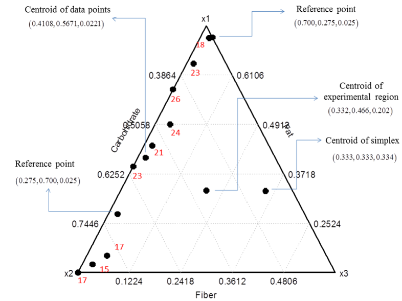
Figure 1.
Realized number (labelled in red) of DMBA-induced tumors in mammary glands of rats treated with different caloric proportions of fiber, fat and carbohydrate on simplex restricted region with reference points.
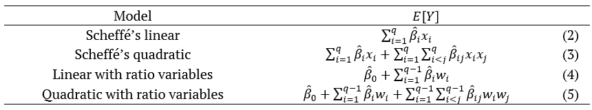
Table 1.
Classifications of the most common mixture models.
Analysing mixture experiments using Dispersion models
Let n independent realizations from a binomial distribution with parameters ni and πi. Assuming that the transformed value of the probability of response to the i-th observation is related to a linear combination of q mixture of components, that is, 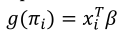 , where g is a the link function and
  is any of the models in Table 1. We adopt g as the logistic transformation. In this case, we have
  , which results in the logistic regression model Equation 6:

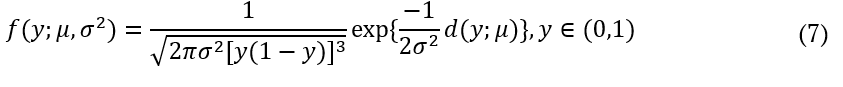
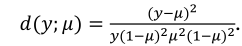
The usual method to estimate  is through Maximum Likelihood. Logistic regression can be used in situations where the response is a Bernoulli event or arises as the proportion of events Y = 1 in n trials and it belongs to the exponential family (Hosmer Jr., Lemeshow, & Sturdivant, 2013) A distribution that can be used to study a variable continuous response restricted to the (0,1) interval is a simplex distribution (Zhang and Qiu, 2014). The simplex distribution is included among dispersion models, which extend the generalized linear models (Barndorff-Nielsen & Jørgensen, 1991;Jørgensen, 1997b;López, 2013;Quintero & Contreras-Reyes, 2018). A random variable y following a simplex distribution with mean μ∈(0,1) and dispersion parameter
  has density function given by Equation 7.
where:
 The distribution of y is denoted by
  For a random sample
  , each
  the simplex regression model is defined by the density of the Equation 7 and the averages
  modeled by
  , where g and
  are as previously defined.
One desirable feature of simplex regression is fitting for heterocaedastic variances. Unlike beta regression model, expected variances are not a function of  . The extra dispersion parameter provides greater flexibility for modeling (Jørgensen, 1997a;Zhang and Qiu, 2014).
The procedure for estimation of the simplex regression model parameters is similar to the logistic regression, with the difference that the additional parameter  should be estimated. The log-likelihood function for n independent observations is given by Equation 8.

The maximum likelihood estimators of parameters  and
and  are obtained through the solution of the homogeneous equations. However, for
  it results in closed form. The estimation of b requires the use of a numerical maximization, usually any method for this works, like Newton-Raphson or Fisher's scoring and its variations (McCulloch et al., 2009).
Selecting models and goodness of fit criterion
Akaike information criterion (AIC) is a relative measure of goodness of fit, defined by 
 , where
  is the (neperian) logarithm of the model likelihood function evaluated at the point estimates
  and p is the number of model parameters. Alternatively, a slight modification of AIC, known as Bayesian Information Criterion (BIC), weights the parameters by
  , where n is sample size (Menezes, Liska, Cirillo, & Vivanco, 2017).
Bozdogan (2010) proposed the information complexity index (ICOMP), which uses the Fisher’s information matrix evaluate model complexity, as this accounts for correlation of parameters’s estimates (Silhavy, Senkerik, Oplatkova, Prokopova, & Silhavy, 2017). The ICOMP is defined as Equation 9.

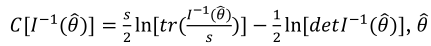 are the parameters estimated,
  the inverse of the Fisher information matrix, and
  . Diagonal elements of
  are estimated variances of model parameters and off-diagonal elements are their covariances. This is a measure of collinearity between columns of
  and the degree of independence of parameters (or their estimates). According to this criterion, the best model within a set of models is the one which minimizes the ICOMP (Bozdogan, 2010).
Goodness of fit can be also checked by a normal probability plot for residuals, a graphical indication that distributional assumptions are violated. This plot, also called envelope simulated chart, contains resampling confidence bands, and it is judged that suitable adjustment has occurred if all model residuals (or at least most of them) are contained within these bands (Moral, Hinde, & Demétrio, 2017) .
Interpreting parameters and measuring the effect of the components in mixture experiments
For mixture experiments with logistic transformation, model coefficients estimates are not directly interpreted as odds ratios, as the restrictions limit interpretation and unexpected interactions may be present. In other words, if the estimate for xi increases, then estimates for other components should decrease, but their ratio to one another remains constant. To better understand this concept, we should use the Cox direction, as explained by Cornell (1998).
Cox direction for trace response plot
The component i of Cox direction is an imaginary line projected from the reference mixture to the vertex xi = 1. The proportions of the q components in the reference mixture are  , where
  . The reference point c default is generally adopted as the centroid of the experiment. When the proportion ci of the component i is changed by an amount Δi toward the Cox direction, then the new ratio becomes Equation 10.

The proportions of the q-1remaining components resulting from ci in the i-th component is Equation 11.

In the case of a restricted experimental region to be a regular simplex, an alternative representation of the Cox direction may be formulated, considering the fact that  . In a mixture system with q=3, along the componentsaxis xj passing through the reference point, the components xjand xk such that
  are given by
  with, pxishows the ratio of the components except xi in the reference point. Thus, the value of the predicted response for the first grade linear predictor, along the Cox direction for the i-th component is given by Equation 12:

In Equation 12, exponentiating  , gives predicted values of
  for each mixture component xi. A plot that relates the increments of xi to the values of
  and this graph is called ‘trace plot’. These lines represent the effect of changing each blend component while all other components remain at constant rates. Model given by equation Equation 12 can be expanded to different linear predictors (Akay, 2007).
Odds ratio plots for mixture components
Odds ratio are used for easy interpretation of parameter’s coefficient estimates in logistic regression (Chen, Cohen, & Chen, 2010). For mixture experiments, techniques based upon trace response graphics can be used for such comparisons. Considering any point c = (c1, c2, ck) taken as a control group on the experimental region, the odds ratio is given along the xi axis by Equation 13.
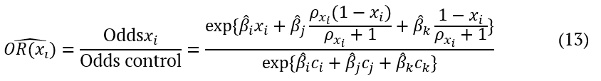
In the simplest way,  . The precision of the odds ratio can be determined by the confidence interval and its range reflects its variability (Hosmer Jr. et al., 2013). Using methods for calculating the variance of a sum, we can obtain estimated variance of the logarithm of the odds ratio. The
  confidence interval is given by Equation 14.

where:
 is the neperian logarithm standard error for the odds ratio and
  standard normal quantile with
  significance level.
Lower and upper limits for odds ratios can be back transformed exponentiating the limits in Equation 14. Narrow confidence intervals are also a criteria for selecting better models or estimation methods. Thus, plotting confidence regions for odds ratios can be also used to compare models.
We used the statistical packages, bbmle (Bolker, 2017) and mixexp (Lawson & Willden, 2016) of R Statistical Computing System (R Core Team, 2018).
Results and discussion
Model selection
Logistic regression results described in Table 2 are identical to Akay and Tez (2011), which presented the model with ratio variables as a better alternative than the logistic regression model with variables in pseudo-components on polynomial models of Scheffé and Backer. Thus, compared to the results obtained by these authors, this indicates that simplex regression model performs better. For models with ratio variables, the lowest values of ICOMP, AIC and BIC criteria were obtained. Therefore, the simplex regression model with ratio variables was the best of the models used and the model provided lower standard errors of the model parameter estimates, indicating more precision.
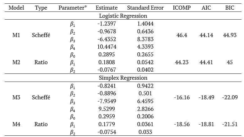
Table 2.
Parameter estimates for the adjusted models and results of adjustment quality indicators.
*Parameters related to Scheffé quadratic model, with linear predictor given by , and Ratio linear, with linear predictor given by .
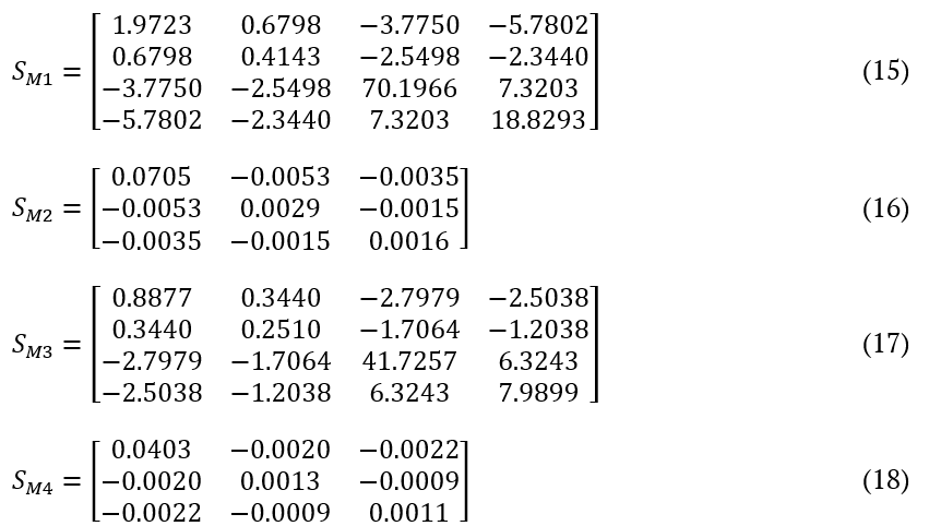
Parameter estimates for the component x3 is larger than the other parameters. Menard (2010) warns that the reason for this discrepancy between the estimates of the model parameters is due to collinearity. This can be seen studying covariance matrices SM1 and SM3 of the models M1 and M3. Diagonal elements of SM3 indicate more precise estimates for models M2 and M4.
The covariances between parameters in the M2 and M4 models are smaller than those of models M1 and M3, as can be seen in the SM2 and SM3 matrices, which provides an explanation for the difference between the ICOMP values. As Bozdogan (2010) mentioned, systems whose covariance between its components are more evident tend to have higher values for ICOMP and, on the other hand, smaller covariance results in lower values for ICOMP. In addition, the M4 model has more information about the parameters, since the variances thereof are smaller than those of other models. Some care is always needed interpreting those models as some coefficients are for ratios of design variables (Equation 15 to 18).
Akay and Tez (2011) addressed the presence of the under or over-dispersion effect on pooled data, such as the data presented in Figure 1 and the authors mentioned that this fact must be taken into account when selecting the model. The estimated dispersion parameters of the M1 and M2 models are 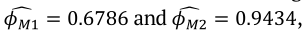 , respectively. In this case, it can be said that the under-dispersion effect in model M1 is present and therefore is missspecified. When using the model with ratio variables (M2), the dispersion parameter estimate is close to the unit value, which is the default value for the usual logistic regression model. Thus, it can be said that the model M2 controlled the under-dispersion effect. In the case of the M3 and M4 models, the simplex regression model naturally models the dispersion and the estimates are given by
 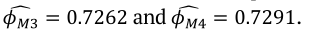 .
.
Given the above, it can be concluded that the simplex regression model showed better adjustment of quality indicators for the proportion of breast tumors in female rats (Table 2). For comparison purposes, the M2 and M4 models have been discussed, since the M2 was the best among the ones proposed by Akay and Tez (2011) and M4 considered the best among simplex distribution. Thus, the normal probability plot of the residual deviation component for the M2 and M4 models supports the claim that the assumption of binomial (Figure 2a) and/or simplex (Figure 2b) response for the analyzed response is adequate and the adjustment of the models were satisfactory (Figure 2).
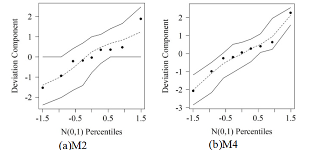
Figure 2.
Simulated envelope for goodness of fit diagnostic of the M2 (a) and M4 (b) models.
Models discussion about the mixture component effect plots
In what follows we describe graphic interpretation of M2 and M4 models. Trace plots for the reference point in Cox direction was given to the centroid c = (0.4108,0.5671,0.0221), as can be seen in Figure 1.
In Figure 3a, M2 model, the x1 (fat) and x2 (carbohydrate) components have opposite effect on the response. As the proportion of fat increases, the expected tumor incidence increases. On the other hand, as the proportion of carbohydrate increases the expected tumor incidence decreases. The x3 (fiber) component has more effect on the response than other components, since successive increments of dietary fiber lead to a higher expected decrease in tumors. Similarly, the same conclusions can be made for the M4 model.
Figure 4 and 5 present the odds ratios for different reference points in relation to the control group for each evaluated model. To this end, we considered three different reference points (0.7, 0.275, 0.025), (0.275, 0.7, 0.025) and (0.332, 0.466, 0.202). The first two points of reference are contained in the region where the sample points lie. The third reference point is the centroid of the constrained experimental region (Figure 1). The control group was given by the centroid of sampling points c = (0.4108,0.5671,0.0221). This work is not adhered to the biological reasons for the choice of these points, but the fact that such choice was made strictly by inspection of the experimental region and applicability in mixture experiments.
Odds are that mammary tumors occurrence increase with larger values in the x1 component. The respective M2 model 95% confidence interval contains the value 1, used to compare the odds ratios in amounts from 0.4 to 0.6 approximately. Therefore although the chance increases to the amounts 0.4 to 0.6, approximately, of x1, it is not significant in the sense that the component in the population x1 (fat) does not significantly influence the occurrence of mammary tumors in rats (Figure 4A).
For point estimates, the same conclusions apply for the x1component in the M4 model. However, we note that the 95% confidence interval for the odds ratio does not contain the value 1 for some values of x1 (Figure 5A), indicating that this component significantly influences the occurrence of mammary tumors in different quantities than those explained by model M2 (Figure 5). This fact is evidenced by the width of the confidence interval for the odds ratio of this component, which is narrower in the M4 model than in the M2 model. Therefore, the M4 model provides estimates of the x1 component more precise than model M2 (Figure 5).
M4 model provided more precise estimates of the odds ratio than the M2 model in all adopted reference points (Figure 4A-C). This fact can be explained by inspection of the covariance between the parameters of the models evaluated. Therefore, we concluded that considering the proportion of mammary tumors incidence in rats as a random variable with simplex distribution, the use of ratio variables to study the relationship between fat, carbohydrate, and fiber mixture components is a viable alternative to the model proposed by Akay and Tez (2011).
Other information that can be provided by the model is the particular mixture that provide the maximum (or minimum) tumor incidence, respecting the constraints of each component. Minimum expected tumor incidence in the model that showed the best fit quality indicators (M4) is 55.08% and the mixture providing this value is formulated as 13.36 fat, 86.34% carbohydrate and 0.30% fiber (Table 3). Major difference on components that maximize or minimize response was achieved varying proportion of fat and carbohydrate in the mixture.
Figure 3.
Trace plots for the M2 (a) and M4 (b) models considering the point c = (0.4108,0.5671,0.0221), the centroid data, as reference point.
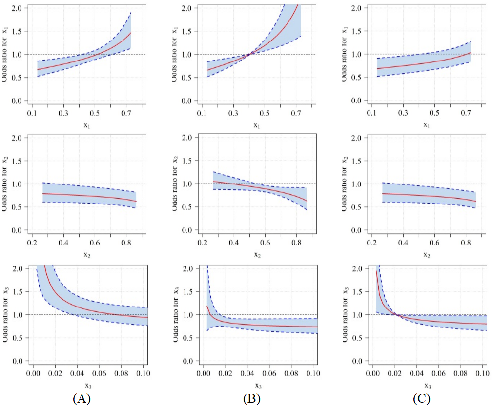
Figure 4.
Odds ratio and their respective 95% confidence interval for the M2 model where (A) the reference point is (0.7, 0.275, 0.025) and control group (0.4108, 0.5671, 0.0221), (B) the reference point is (0.275, 0.7, 0.025) and control group (0.4108, 0.5671, 0.0221) and (C) the reference point is (0.332, 0.466, 0.202) and control group (0.4108, 0.5671, 0.0221).

Figure 5.
Odds ratio and their respective 95% confidence interval for the M4 model where (A) the reference point is (0.7, 0.275, 0.025) and control group (0.4108, 0.5671, 0.0221), (B) the reference point is (0.275, 0.7, 0.025) and control group (0.4108, 0.5671, 0.0221) and (C) the reference point is (0.332, 0.466, 0.202) and control group (0.4108, 0.5671, 0.0221).
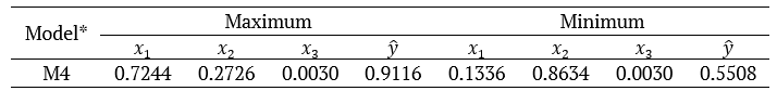
Table 3.
Mixture of components x1 (fat), x2 (carbohydrate) and x3 (fiber) that provides the maximum and minimum expected incidence of tumor (ŷ ).
M4 (Simplex Regression ratio type).
Conclusion
Simplex regression model showed good fit to the analysis of a mixture experiment that evaluated the incidence of mammary tumors in female rats, being a viable option in the analysis of situations where the outcome is limited to the (0,1) interval. The use of this model also accounts for the under or over-dispersion present in grouped data.
Confidence intervals for the odds ratio were severely affected by choices of reference points. The simplex regression model provided more precise estimates for the odds ratio (narrower confidence limits). The model gave more stable estimates for odds ratios in different reference points in the experimental region, compensating for border effect.
References
Akay, K. U. (2007). A note on model selection in mixture experiments. Journal of Mathematics and Statistics, 3(3), 93-99. doi: 10.3844/jmssp.2007.93.99
Akay, K. U., & Tez, M. (2011). Alternative modeling techniques for the quantal response data in mixture experiments. Journal of Applied Statistics, 38(11), 2597-2616. doi: 10.1080/02664763.2011.559214
Barndorff-Nielsen, O. E., & Jørgensen, B. (1991). Some parametric models on the simplex. Journal of Multivariate Analysis, 39(1), 106-116. doi: 10.1016/0047-259X(91)90008-P
Dal Bello, L. H. A., & Vieira, A. F. C. (2011). Tutorial for mixture-process experiments with an industrial application. Pesquisa Operacional, 31(3), 543-564. doi: 10.1590/S0101-74382011000300008
Bolker, B. (2017). Tools for general maximum likelihood estimation. Retrived from: https://cran.r-project.org/web/packages/bbmle/bbmle.pdf
Bozdogan, H. (2010). A new class of information complexity (ICOMP) criteria with an application to customer profiling and segmentation. İstanbul Üniversitesi İşletme Fakültesi Dergisi, 39(2), 370-398.
Brown, L., Donev, A. N., & Bissett, A. C. (2015). General blending models for data from mixture experiments. Technometrics, 57(4), 449-456. doi: 10.1080/00401706.2014.947003
Chen, H., Cohen, P., & Chen, S. (2010). How big is a big odds ratio? interpreting the magnitudes of odds ratios in epidemiological studies. Communications in Statistics - Simulation and Computation, 39(4), 860-864. doi: 10.1080/03610911003650383
Cornell, J. A. (1998). Chapter 25 mixture designs. In D. L. Massart, B. G. M. Vandeginste, L. M. C. Buydens, S. Jong, P. J. Lewi, & J. Smeyers-Verbeke (Eds.), Handbook of chemometrics and qualimetrics: part A (p. 739-769). Amsterdam, NL: Elsevier Science.
Cruz-Salgado, J. (2016). Comparing the intercept mixture model with the slack-variable mixture model. Ingeniería, Investigación y Tecnología, 17(3), 383-393. doi: 10.1016/j.riit.2016.07.008
Pawlowsky-Glahn, V., Egozcue, J. J., & Tolosana-Delgado, R. (2015). Modeling and analysis of compositional data. Chichester, EN: John Wiley & Sons.
Hosmer Jr., D. W., Lemeshow, S., & Sturdivant, R. X. (2013). Applied logistic regression (3rd ed). Hoboken, NJ: John Wiley & Sons.
Jørgensen, B. (1997a). Proper dispersion models. Brazilian Journal of Probability and Statistics, 11(2), 89-128.
Jørgensen, B. (1997b). The theory of dispersion models. London, UK: Chapman & Hall.
Lawson, J., & Willden, C. (2016). Mixture experiments in R using mixexp. Journal of Statistical Software, 72(2), 1-20. doi: 10.18637/jss.v072.c02
Leão, M. N. S., Vieira, A. F. C., & Dal Bello, L. H. A. (2015). A model selection procedure in mixture-process experiments for industrial process optimization. Pesquisa Operacional, 35(2), 377-399. doi: 10.1590/0101-7438.2015.035.02.0377
Liska, G. R., Silveira, E. C., Reis, P. R., Cirillo, M. A., & Gonzalez, G. G. H. (2015). Selecting a binomial regression model on the predation rate of euseius concordis (Chant, 1959). Coffee Science, 10(1), 113-121. doi: 10.25186/cs.v10i1.786
López, F. O. (2013). A bayesian approach to parameter estimation in simplex regression model: a comparison with beta regression. Revista Colombiana de Estadística, 36(1), 1-21. doi: 10.15446/rce
McCulloch, C. E., Searle, S. R., & Neuhaus, J. M. (2009). Generalized, linear, and mixed models (2nd ed.). New York: John Wiley & Sons.
Menard, S. W. (2010). Logistic regression: from introductory to advanced concepts and applications. London, UK: Sage Publications.
Menezes, F. S., Liska, G. R., Cirillo, M. A., & Vivanco, M. J. F. (2017). Data classification with binary response through the Boosting algorithm and logistic regression. Expert Systems with Applications, 69, 62-73. doi: 10.1016/j.eswa.2016.08.014
Moral, R. A., Hinde, J., & Demétrio, C. G. B. (2017). Half-normal plots and overdispersed models in r: the hnp package. Journal of Statistical Software, 81(10), 1-23. doi: 10.18637/jss.v081.i10
Quintero, F. O. L., & Contreras-Reyes, J. E. (2018). Estimation for finite mixture of simplex models: applications to biomedical data. Statistical Modelling, 18(2), 129-148. doi: 10.1177/1471082X17722607
R Core Team. (2018). R: A language and environment for statistical computing. Vienna, AT: R Core Team.
Silhavy, R., Senkerik, R., Oplatkova, Z. K., Prokopova, Z., & Silhavy, P. (2017). Artificial intelligence trends in intelligent systems. Cham, SW: Springer.
Zeviani, W. M., Ribeiro Jr., P. J., Bonat, W. H., Shimakura, S. E., & Muniz, J. A. (2014). The gamma-count distribution in the analysis of experimental underdispersed data. Journal of Applied Statistics, 41(12), 2616-2626. doi: 10.1080/02664763.2014.922168
Zhang, P., & Qiu, Z. (2014). Regression analysis of proportional data using simplex distribution. Scientia Sinica Mathematica, 44(1), 89-104. doi: 10.1360/012013-200
Notas de autor
gilbertoliska@ufscar.br