1. Introduction

The Lie group symmetry method emerges as a potent tool employed for the analy-sis of differential equations (DEs), encompassing both ordinary differential equations (ODEs) and partial differential equations (PDEs), as well as fractional differential equa-tions (FDEs) and various other equation types. This theory, originating in the 19th century by the mathematician Sophus Lie [1], follows in the footsteps of Galois theory within the realm of algebra. The application of the Lie group method to differential equations has engendered considerable interest across a spectrum of scientific disciplines, including pure mathematics and both theoretical and applied physics. This stems from the invaluable physical interpretations it affords to the scrutinized equations. Conse-quently, this approach facilitates the construction of conservation laws, employing, for instance, the renowned Noether’s Theorem [2], and even symmetry solutions, a feat unattainable through conventional methods.

Moreover, this method contributes to the formulation of frameworks and the assessment of numerical methods, among other applications [3, 4, 5]. Present-day Lie symmetries have undergone extensive scrutiny, as evidenced by the comprehensive body of work available in the literature [6, 7, 8, 9, 10].

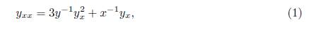
Within the study of the diffusions, specifically in the study of a relativistic fluid sphere by considering the so-called isotropic metric, Buchdahl [11] obtained the equation

the solution of which is,

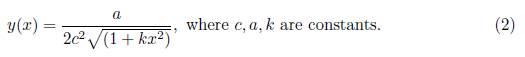
In [12], the first three integrals of (1) are presented using the Prelle-Singer method. In [13], first integrals of (1) are also derived by employing the relation between sym-metries and extending the Prelle-Singer method. In [14], the first integrals of (1) are obtained through an extension of the Prelle-Singer method. All of the aforementioned authors have arrived at the same solution for (1)

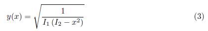
where I₁ and I₂ are first integrals. It is worth noting that (2) and (3) are equivalent when the constants are arranged accordingly. In [15], Zaitsev and Polyanin present a solution to (1)

The primary objectives of this article are as follows: We will begin by presenting the 5 dimensional Lie symmetry group for (1), offering a comprehensive description of its computation. Next, we will utilize this Lie symmetry group to introduce an optimal system, also known as an optimal algebra, for (1). Using the elements of the optimal system, we will then proceed to derive invariant solutions for (1). Following this, we will construct the Lagrangian associated with equation (1), based on the calculated group of symmetries. This will enable us to determine variational symmetries through the application of Noether’s theorem, ultimately leading to the presentation of associated conservation laws. Furthermore, we will employ Ibragimov’s method to establish non-trivial conservation laws. Finally, leveraging the group of symmetries we have identified, we will undertake the classification of the Lie algebra associated with (1).

2. About the Lie group symmetries for relativistic fluid sphere equa-tion.

The purpose of this section is to determine for (1) the group of Lie symmetries. This objective is explained in the following proposition

Proposition 2.1. The Lie group of symmetries for theequation (1)consists of the fol-lowing elements:

And Γ₅ = x²y³ $\frac{\partial }{\partial \gamma }.$

Proof. The general form for the generator operators of a Lie group with an admissible parameter for (1) is as follows:

where is the group parameter. The vector field associated with this group of transfor-mations is given by:

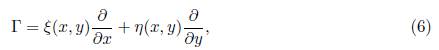
with ξ and η being differentiable functions in ℝ². To calculate the infinitesimals η and ξ in (6), we employ the second extension operator

to the equation (1), resulting in the following symmetry condition:

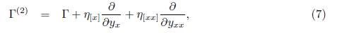
where η [x] and η[xx] are the coefficients in Γ² given by:

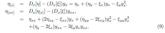
where D_x is the total derivative operator: D_x = ∂_x + y_x∂_y + y_xx∂_yx + .

After applying (9) to (8) and substituting the resulting expression for y_xx with (1), we obtain the following:

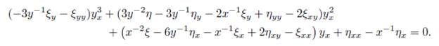
after analyzing the coefficients in regard to the independent variables y_x³; y_x²; y_x; 1 we get the following system of determining equations:

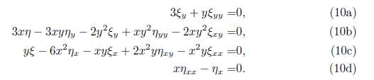
Solving in (10a) and (10d) we get

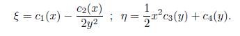
Using these equations in (10b) and (10c) to solve for c₁(x); c₂(x); c₃(y), and c₄(y), we obtain the following:

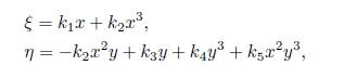
where k₁; k₂; k₃; k₄, and k₅ are arbitrary constants. Thus, by usingand in the operator (6) and grouping the constants, we obtain Γ₁ through Γ₅, which constitute the generators of the symmetry group for the equation (1), as proposed in the statement of Proposition 2.1.

3. About optimal system

Considering [16, 18, 19, 20, 21, 17], we will now present the optimal system for (5). To determine the optimal algebra, it is essential to first obtain the corresponding commutator table. This can be calculated using the following operator:

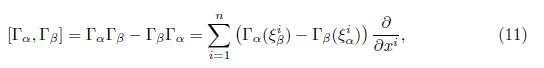
where i = 1; 2, with α, β = 1; …; 5 and ξⁱ_α; ξⁱ_β are the corresponding coefficients of the Γ_α, Γ_β:

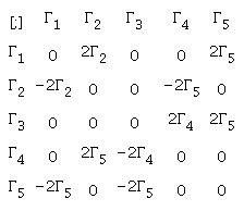
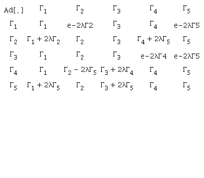
In Table 1, we present the results obtained by applying the operator (11) to the symmetry group (1).

Following the objective for determining the optimal algebra, we must now obtain the ‘Adjoint Representation’ using Table 1 and the next operator (Ad):

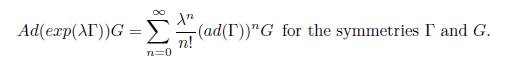
In Table 2, we display the adjoint representation for each Γ i, with each entry in this table calculated using the operator mentioned above.

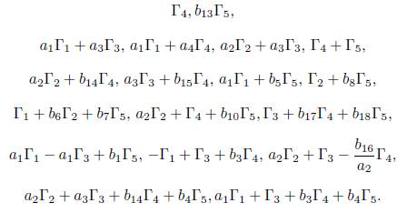
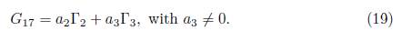
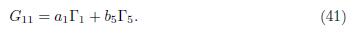
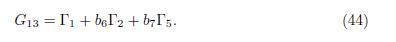
Proposition 3.1. The vector fields that represent the optimal algebra associated with the equation (1) are as follows:

Proof. Considering the generic operator G, which is a linear combination of the symmetry group (5). Let

Using the adjoint operator (Ad) in G and the elements from Table 2, we can simplify the coefficients α_i as much as possible, which will be our goal at every step of this proof.

1) Assuming α₅ = 1 in (12) we have that G = α₁Γ₁ + α₂Γ₂ + α₃Γ₃ + α₄Γ₄ + Γ₅. Using the adjoint operator to (Γ₁; G) and (Γ₃; G) no reductions are available, but applying the adjoint operator to (Γ₂; G) we obtain

1.1) Case α₁ # 0. applying λ₁ = $\frac{{-a}_2}{{2a}_3}$ with α₁ # 0, in (13), Γ₂ is eliminated, therefore G₁ = α₁Γ₁ + α₃Γ₃ + α₄Γ₄ + b₁Γ₅, where b₁ = 1 - $\frac{a_2{a}_4}{a_1}$. Now, using the adjoint operator to (Γ₄, G₁), we obtain G₂ = Ad (exp (λ₂ Γ₄)) G₁ = α₁Γ₁ + α₃Γ₃ + (α₄ + 2α₃λ₂) Γ₄ + b₁Γ₅.

1.1.A) Case α₃ # 0. Using λ₂ =$\frac{{-a}_4}{{2a}_3}$, with α₃ # 0, is eliminated Γ₄, then G₂ = α₁Γ₁+ α₃Γ₃ + b₁Γ₅. Using the adjoint operator to (Γ₅, G₂), we obtain

1.1.A.A₁) Case α₁ + α₃ # 0. Using λ₃= - $\frac{b_1}{2({\alpha }_1+{\alpha }_3)}$, with α₁ + α₃ # 0, in (14), Γ₅ is eliminated, therefore G₃ = α₁Γ₁+ α₃Γ₃. This is how the first optimal element appears

Then, we obtain the first reduction of the generic element (12).

1.1. A.A₂) Case α₁ + α₃ = 0. We get in (14), G₃ = α₁Γ₁ - α₁Γ₃ + b₁Γ₅. This is how the other optimal element appears

Then, we obtain one more reduction of the generic element (12).

Case α₃ = 0. We get, G₂ = α₁Γ₁ + α₄Γ₄ + b₁Γ₅. Now, applying the adjoint operator to (Γ₅,G₂), we have G₁₅ = Ad (exp(λ₁₅Γ₅)) G₂ = α₁Γ₁ + α₄Γ₄ + (b₁ + 2α₁λ₁₅)Γ₅. Then, as Γ₁ = 0, we can substitute λ₁₅ = $\frac{{-b}_1}{2_{\alpha 1}}$, then Γ₅ is removed, then an another item of the optimal algebra is

1.2) Case α₁ = 0. Now, we have, G₁ = α₂Γ₂ + α₃Γ₃ + Γ₄ + (1 + 2α₄λ₁)Γ₅.

1.2. A) Case α₄ # 0. Using λ₁ = $\frac{-1}{2_{\alpha 4}}$ with α₄ # 0, Γ₅ is removed, therefore G₁= α₂Γ₂ + α₃Γ₃ + Γ₄. Now, applying the adjoint operator to (Γ₄, G₁), we get

1.2.A.A₁) Case α₃ # 0. Using λ₁₆ = $\frac{-1}{2_{\alpha 3}}$ with α₃ # 0, Γ₄ is eliminated, therefore G₁₆ = α₂Γ₂ + α₃Γ₃ + b₉Γ₅, where b₉ = $\frac{{\mathrm{\alpha }}_2}{{\mathrm{a}}_3}$. Now, using the adjoint operator to (Γ₅,G₁₆), we obtain

Then, α₃ # 0, we can substitute λ₁₇ = $\frac{{-b}_9}{2_{\alpha 3}}$, then Γ₅ is removed, after we get other item

1:2:A:A₂) Case α₃ = 0. We get in (18), G₁₆ = α₂Γ₂ + Γ₄ - 2 α₂λ₁₆Γ₅.

1:2:A:A₂:1) Case α₂ 6= 0. Applying λ₁₆= $\frac{{-b}_{10}}{2_{\alpha 2}}$ with α₂ # 0, we get G₁₆ = α₂Γ₂ + Γ₄ + b₁₀Γ₅. Now, applying the adjoint operator to (Γ₅;G₁₆), it is not possible to further reduce, this is how the other optimal element appears:

1:2:A:A₂:2) Case α₂ = 0. We have G₁₆ = Γ₄. Now, using the adjoint operator to (Γ₅;G₁₆), Therefore, there are no reductions, this is how the other optimal element appears:

1:2:B) Case α₄ = 0. We get, G₁ = α₂Γ₂ + α₃Γ₃ + Γ₄ + Γ₅. Now, applying the adjoint operator to (Γ₄;G₁), we have

1:2:B:1) Case α₃ # 0. Using λ₁₉ = $\frac{-1}{2_{\alpha 3}}$, with α₃ # 0, Γ₄ is eliminated, therefore G₁₉ = α₂Γ₂ + α₃Γ₃ + b₁₁Γ₅, with b₁₁ = 1 + $\frac{a2}{a3}$. Now, using the adjoint operator to (Γ₅;G₁₉), we obtain

Then, as α₃ # 0, we can substitute λ₂₀ = $\frac{{-b}_{11}}{2_{\alpha 3}}$, then Γ₅ is removed, after we get other item of the optimal algebra

Then, we obtain one more reduction of the generic element (12).

1:2:B:2) Case α₃ = 0. We have in (22), G₁₉ = α₂Γ₂ + Γ₄ + (1 - 2α₂λ₁₉)Γ₅.

1:2:B:2:A1) Case α₂ # 0. Using λ₁₉ = $\frac{1}{2_{a2}}$, with α₂ # 0, Γ₅ is eliminated, therefore G₁₉ = α₂ Γ₂+Γ₄. Now, applying the adjoint operator to (Γ₅;G₁₉), it is not posible to further reduce, this is how the other optimal element appears

1:2:B:2:A2) Case α₂ = 0. We get G₁₉ = Γ₄ + Γ₅. Now, applying the adjoint operator to (Γ₅;G₁₉), it is not possible to further reduce, this is how the other optimal element appears:

2) Assuming α₅ = 0 and α₄ = 1 in (12), we have that G = α₁Γ₁ + α₂Γ₂ + α₃Γ₃ + Γ₄. Using the adjoint operator to (Γ₁;G) and (Γ₃;G) and there is no reduction, but applying the adjoint operator to (Γ₂;G) we obtain

2:1) Case α₁ # 0. Using λ₄ = $\frac{{-a}_2}{2_{a1}}$, with α₁ # 0, in (27), Γ₂ is eliminated, therefore G₄ = α₁Γ₁ + α₃Γ₃ + Γ₄+ b₂Γ₅, where b₂ = λ₄ = $\frac{{-a}_2}{2_{a1}}$. Now, using the adjoint operator to (Γ₄, G₄), we obtain G₅ = Ad (exp (λ₅Γ₄)) G₄ = α ₁Γ₁ + α ₃Γ₃ + (1 + 2 α ₃λ₅)Γ₄ + b₂Γ₅.

2.1.A) Case α₃ # 0. Using λ₅ = $\frac{-1}{2_{a3}}$ with α₃ # 0, Γ₄ is eliminated, therefore G₅ = α ₁Γ₁ + α₃Γ₃ + b₂Γ₅. Now, using the adjoint operator to (Γ₅, G₅), we obtain G₆ = Ad (exp (λ₆Γ₅)) G₅ = α₁Γ₁ + α₃Γ₃ + (b₂ + 2λ₆(α₁ + α₃))Γ₅

2:1:A:A₁) Case α₁ + α₃ # 0. Using λ₆ = $\frac{b_2}{2_{(a1+a3)}}$ with α₁ + α₃# 0, Γ₅ is eliminated, therefore G₆ = α₁Γ₁ + α₃Γ₃. This is how the other optimal element appears:

2.1.A.A₂) Case α₁ + α ₃ = 0. we get G₆ = α ₁Γ₁-α ₁Γ₃ + b₂Γ₅. This is how the other optimal element appears:

2.1.B) Case α₃ = 0. We have G₅ = α₁Γ₁ + Γ₄ + b₂Γ₅. Now, applying the adjoint operator to (Γ₅, G₅), we have G₂₁ = Ad (exp (λ₂₁Γ₅)) G₅ = α₁Γ₁ + Γ₄ + (b₂ +2 α₁λ₂₁)Γ₅. Then, as αa₁ # 0, we can substitute λ₂₁ = $\frac{-b_2}{2_{a1}}$, then Γ₅ is removed, after we get another item of the optimal algebra

2.2) Case α₁ = 0. We have in (27), G₄ = α₂Γ₂ + α₃Γ₃ +Γ₄ + 2λ₄Γ₅, using λ₄ = $\frac{b_{1a}}{2}$, get G₄ = α₂Γ₂ + α₃Γ₃ + Γ₄ + b₁₃Γ₅. Now, using the adjoint operator to (Γ₄, G₄), we obtain G₂₁ = Ad (exp (λ₂₁Γ₄)) G₄ = α₂Γ₂ + α₃Γ₃ + 2 α₃λ₂₁Γ₄ +(b₁₃ − 2α₂λ₂₁)Γ₅.

2.2.A) Case α₂ # 0. Using $\frac{b_{1a}}{a_2}$, with α₂ # 0, Γ₅ is eliminated, therefore G₂₁ = α₂Γ₂ + α₃Γ₃ + b₁₄, where b₁₄ = $\frac{a_3{b}_{13}}{a2}$ . Now, using the adjoint operator to (Γ₅, G₂₁), we obtain

2:2:A:1) Case α₃ # 0. It is clear that is not possible to further reduce, then using λ₂₂ = $\frac{b_{15}}{2a_3}$, with α₃ # 0, this is how the other optimal element appears:

Then, we obtain one more reduction of the generic element (12).

2:2:A:2) Case α₃ = 0. We obtain G₂₂ = α₂Γ₂ + b₁₄Γ₄. This is how the other optimal element appears:

2:2:B) Case α₂ = 0. We have G₂₁ = α₃Γ₃ + 2α₃λ₂₁Γ₄ + b₁₃Γ₅.

2:2:B:1) Case α₃0. Using λ₂₁ = $\frac{b_{15}}{2a3}$, we get G₂₁ = α₃Γ₃ + b₁₅Γ₄ + b₁₃Γ₅. Now, applying the adjoint operator to (Γ₅, G₂₁) we have

Then, as α ₃ # 0, we can substitute λ₂₃ = $\frac{b_{13}}{2a3}$, then Γ₅ is removed, after we get another item of the optimal algebra

2:2:B:2) Case α₃ = 0. We have G₂₁ = b₁₃Γ₅. Now, using the adjoint operator to (Γ₅, G₂₁), therefore, there are not any more reductions. This is how the other optimal element appears:

3)Assuming α₄ = α₅ = 0 and α₃ = 1 in (12), we have that G = α₁Γ₁+ α₂Γ₂+Γ₃. Using the adjoint operator to (Γ₁, G) and (Γ₃, G) there is no reduction, but applying the adjoint operator to (Γ₂, G) we obtain

3:1) Case α₁ # 0. Using λ₇ = $\frac{{-a}_2 }{2a1}$ with α₁ # 0, in (35), Γ₂ is eliminated, therefore G₇ = α₁Γ₁ + Γ₃. Now, using the adjoint operator to (Γ₄;G₇), we obtain G₈ = Ad (exp (λ₈Γ₁))G₇ = α₁Γ₁ + Γ₃ + 2λ₈ Γ₄. It is clear that is not possible to further reduce, then substituting λ₈ = $\frac{b_3 }{2}$ then G₈ = α₁Γ₁ + Γ₃ + b₃Γ₄. Using the adjoint operator to (Γ₅;G₈), we obtain

3:1:A) Case 1 + α₁ # 0. It is clear that it is not possible to further reduce. Then substituting λ₉= $\frac{b_4 }{2(1+a1)}$, this is how the other optimal element appears:

3:1:B) Case 1 + α1 = 0. We have G₉ = - Γ₁ + Γ₃ + b₃Γ₄, then we have other element of the optimal algebra

3.2) Case α₁ = 0. We have G₇ = α₂Γ₂ + Γ₃. Now, using the adjoint operator to (Γ₄, G₇), we get G₂₄ = Ad (exp (λ₂₄Γ₄)) G₇ = α₂Γ₂ + Γ₃ + 2λ₂₄Γ₄ − 2a₂λ₂₄Γ₅.

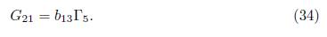
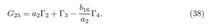
3.2.A₁) Case α₂ # 0. It is clear that is not possible to further reduce, then substituting λ₂₄ = $\frac{{-b}_{16} }{2a2}$, we get G₂₄ = α₂Γ₂ + Γ₃ $\frac{b_{16} }{a2}$Γ₄ + b₁₆Γ₅. Now, using the adjoint operator to (Γ_5,G₂₄₎, we obtain

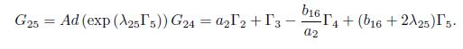
Using λ₂₅ = $\frac{{-b}_{16} }{2}$, Γ₅ is removed, this is how the other optimal element appears:

3:2:A₂) Case α₂ = 0. We have G₂₄ = Γ₃ + 2λ₂₄Γ₄. Using λ₂₄ = $\frac{b_{17} }{2}$, we obtain G₂₄ = Γ₃ + b₁₇Γ₄. Now, using the adjoint operator to (Γ₅; G₂₄), we obtain

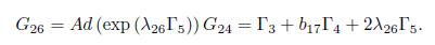
Thus, we do not get any more reduction, then using λ₂₆ = $\frac{b_{18} }{2}$ this is how the other optimal element appears:

4) Using α₃ = α₄ = α₅ = 0 and α₂ = 1 in (12), we obtain that G = α₁Γ₁ + Γ₂. Using the adjoint operator to (Γ₁;G) and (Γ₃;G) we conclude that there is no reduction, but using the adjoint operator to (Γ₂;G) we obtain

4:1) Case α₁ # 0. Using λ₁₀ = $\frac{-1}{{2a}_1}$ $$with a1 # 0, in (40), Γ₂ is eliminated, therefore G₁₀ = α₁Γ₁. Now, applying the operator (Γ₄;G₁₀), it is clear that is not possible to further reduce, but using the adjoint operator to (Γ₅;G₁₀), we obtain G₁₁ = Ad (exp (λ₁₁Γ₅))G₁₀ = α₁Γ₁ + 2 α 1λ₁₁Γ₅. Thus, we do not get any more reduction, then using λ₁₁= $\frac{b_5}{{2a}_1}$, this is how the other optimal element appears:

4:2) Case α₁ = 0. We have G₁₀ = Γ₂. Now, using the operator (Γ₅;G₁₀), it is not possible to further reduce; however, by applying the adjoint operator to (Γ₄;G₁₀), we get

Thus, it is not possible to further reduce it, then using λ₁₄ = $\frac{{-b}_8}{2}$, this is how the other optimal element appears:

5) Using α₂ = α₃ = α₄ = α₅ = 0 and α₁ = 1 in (12), we obtain that G = Γ₁. Applying the adjoint (Adj) to (Γ₁;G) , (Γ₃;G) and (Γ₄;G) it is not possible to further reduce, but applying the adjoint operator to (Γ₂;G) we obtain

it is not possible to further reduce, then substituting λ₁₂ = $\frac{b_6}{2}$ we have that G₁₂ = Γ₁ + b₆Γ₂. Using the adjoint operator to (Γ₅;G₁₂), we obtain

It is not possible to further reduce, then substituting λ₁₃ = $\frac{b_7}{2}$, this is how the other optimal element appears:

4.About invariant solutions

We will characterize the invariant solutions using the operators from Proposition 3.1. To achieve this objective, we will apply the technique of the invariant curve condition ([17], Section 4.3; see also [22]), which is as follows:

An example will be presented below: by taking the element₄ from Proposition 3.1 in (45), we get Q = η₄ y_xξ₄ = 0, then (y³) y_x(0) = 0, thus y(x) = 0, which is the trivial solution for (1).

Table 3 presents both implicit and explicit solutions obtained following the procedure described in the previous paragraph for each element of Proposition (3.1).

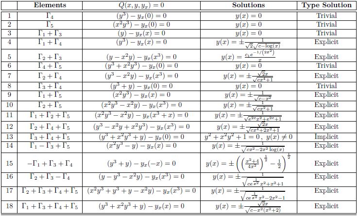
Remarks : Note that the solution in numeral 10 coincides with a particular solution presented in [11]. The solution in numeral 9 coincides with the solution presented in [12] and [14].

5.On the calculation of variational symmetries and the presentation of conserved quantities

We will calculate the variational symmetries of (1), and using Noether’s theorem [2], we will present the conserved quantities.

According to Nucci [23], our first step will be to use the Jacobi Last Multiplier method to calculate the inverse of the determinant Δ with the ultimate goal of obtaining the

Lagrangian.

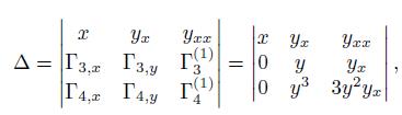
where Γ_4,x, Γ_4,y, Γ_3,x, and Γ_3,y are the components of the symmetries Γ₃ and Γ₄ presented in Proposition 5, and Γ₄¹, Γ₃¹ as their first prolongations. Then, we have ∆ = 2y³y_x , thus M = $\frac{1}{∆}$ = $\frac{y^{-3}}{{2y}_x}$ . According to [23], M = L_yxyx, so L_{yxyx =} $\frac{y^{-3}}{{2y}_x}$ $.$ After integrating twice with respect to yx, we obtain the following Lagrangian:

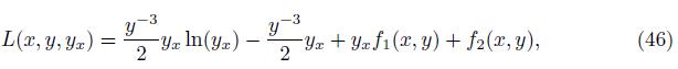
with arbitrary functions f₁ and f₂. In (46), consider f₁ = f₂ = 0. (Note: other Lagrangians can be calculated for (1) using different vector fields in Proposition 5). Thus, we obtain the following:

Applying (46) and (9), we have the following:

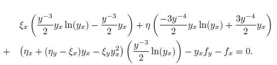
In the last equation, associating terms in regard to 1; y_x; y_x² and y_x³; and simplifying some terms we obtain the following determinant equations:

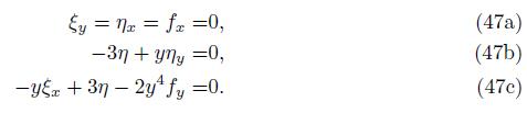
If we solve the system (47a), (47b) and (47c) for ; and f, we obtain the generators of the variational Noether’s symmetries, these solutions are

where α₁; α₂; α₃ and a₄ are constants. Thus, the Noether symmetry group or variational symmetries are

Remarks : Note that V1 = Γ₄ and V2 = Γ₁, this implies that, two of the symmetries of equation (1), are variational symmetries. If we follow what is proposed in [24], the way to calculate the conserved quantities is to solve the expression

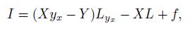
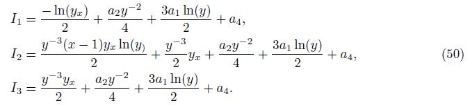
so, using (46), (48) and (49). Therefore, the conserved quantities are given by

6. About Nonlinear Self-Adjointness

In this section, we present the main definitions in N. Ibragimov’s approach to nonlinear self adjointness of differential equations adopted to our specific case. For further details the interested reader is directed to [25, 26, 27].

Consider second order differential equation

with independent variables x and a dependent variable y, where y₍₁₎; y₍₂₎; y_(s) the collection of 1; 2;…; s -th order derivatives of y:

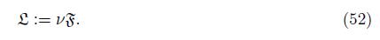
Definition 6.1. Let ℒ be a differential function and = (x)-the new dependent variable, known as the adjoint variable or nonlocal variable [27]. The formal Lagrangian for ℒ = 0 is the differential function defined by

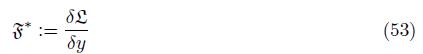
Definition 6.2. Let ℒ be a differential function and for the differential equation (51), denoted by ℒ[y] = 0, we define the adjoint differential function to ℒ by

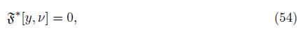
and the adjoint differential equation by

where the Euler operator

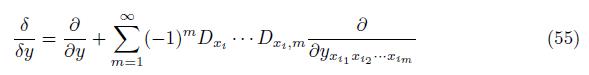
and D_xi is the total derivative operator with respect to x_i defined by

Definition 6.3. The differential equation (51) is said to be nonlinearly selfadjoint if there exists a substitution

such that

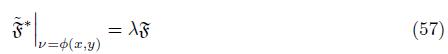
for some undetermined coefficient λ = λ(x, y, · · · ). If ν = φ(y) in (56) and (57), the equation (51) is called quasi self-adjoint. If ν = y, we say that the equation (51) is strictly self-adjoint.

Now we shall obtain the adjoint equation to the eq. (1). For this purpose we write (1) in the form (51), where

Then the corresponding formal Lagrangian (52) is given by

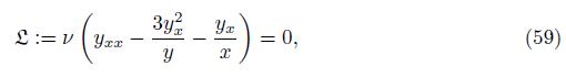
and the Euler operator (55) transfomed into:

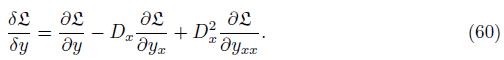
Now, the explicit form of the operator (60), which was applied to ℒ, have the form (59).

Thus, we get the adjoint equation (54) for (1):

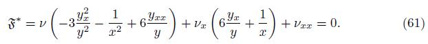
The following proposition presents the most important result of the current section.

Proposition 6.4. The following substitution (x; y) makes equation (1) nonlinearly self-adjoint

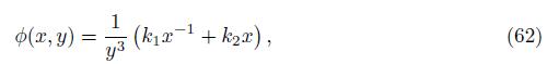
where k₁; k₂are arbitrary constants.

Proof. Substituting in (61), and then in (58), v= $\phi$(x; y) and its respective derivatives, and comparing the corresponding coefficients we get five equations:

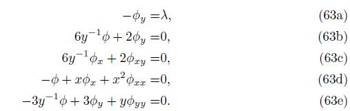
Now, we studies only Eqs. (63b),(63d) and (63e) because the Eq.(63c) is obtaned from

Eq.(63b) by differentiation with respect to x:

When solving the system (63a)-(63e) for $\phi$ we obtain

Then the proposition is proved.

7. About conservation laws

In this section, using the conservation theorem of N. Ibragimov in [27], we will establish some conservation laws for (1). Since the Eq. (1) is of second order, the formal Lagrangian contains derivatives up to order two. Thus, the general formula in [27] for the component of the conserved vector is reduced to

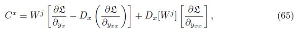
Where

j = 1; ; 5 the formal Lagrangian (59)

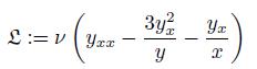
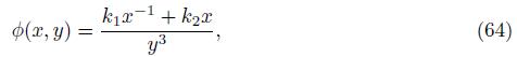
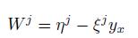
and η^j, ξ^j are the infinitesimals of a Lie group symmetry admitted by Eq. (1), stated in (5). From (1), (5) and (62) into (65) we get the following conservation vectors for each symmetry indicated in (5).

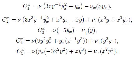
where = y^-3 k₁x^-1 + k₂x and v_{x =} y^-3 (k₁x^-1 + k₂x)

8. Classification of Lie algebra

Using Levi’s theorem, it is possible to classify a finite-dimensional Lie algebra with char-acteristic 0. Also, this theorem makes it possible to deduce the existence of two important classes of Lie algebras: The solvable algebra and the semisimple algebra. As it is known, for the mentioned algebras, there are certain particularities, for example, within the soluble ones there are the Nilpotent Lie algebras.

If we look at the group of generators present in the Table 1, we get a five dimensional Lie algebra. A basic and classical way to classify a Lie algebra is by means of the Cartan-Killing form, which is denote as K(:;:), this form is expressed in accordance with the following propositions [28].

Proposition 8.1. (Cartan’s theorem) A Lie algebra is semisimple if and only if its Killing form is nondegenerate.

Proposition 8.2. A Lie subalgebra g is solvable if and only if K(X; Y ) = 0 for all X 2 [g; g] and Y 2 g. Other way to write that is K(g; [g; g]) = 0.

We also need the next statements to make the classification.

Definition 8.3. Let g be a finite-dimensional Lie algebra over an arbitrary field k. Choose a basis e_j , 1 ≤ i ≤ n, in g where n = dim g and set [e_i, e_j ] = C_ij^ke_k . Then the coefficients C_ij^k are called structure constants.

Proposition 8.4. Let g₁and g₂be two Lie algebras of dimension n. Suppose each has a basis with respect to which the structure constant are the same. Then g₁and g₂are isomorphic.

Let be g the Lie algebra related to the group of infinitesimal generators of the equation (1). Analyzing the table of the commutators (Table 1), it is enough to consider the next relations:

[Γ₁, Γ₂] = 2Γ₂, [Γ₁, Γ₅] = 2Γ₅, [Γ₂, Γ₄] = -2Γ₅, [Γ₃, Γ₄] = 2Γ₄, [Γ₃, Γ₅] = -2Γ₅.

The matrix form of the Cartan-Killing K representation is:

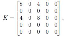
which the determinant vanishes, and thus by Cartan criterion it is not semisimple, (see Proposition 8.1). Since a nilpotent Lie algebra has a Cartan-Killing form that is identi- cally zero, we conclude, using the counter-reciprocal of the last claim, that the Lie algebra g is not nilpotent. We verify that the Lie algebra is solvable using the Cartan criteria to solvability, (Proposition 8.2), and then we have a solvable nonnilpotent Lie algebra. The Nilradical of the Lie algebra g is generated by Γ₂, Γ₄, Γ₅, that is, we have a Solvable Lie algebra with three dimensional Nilradical. Let m the dimension of the Nilradical M of a Solvable Lie algebra. In this case, in fifth dimensional Lie algebra we have that 2 ≤ m ≤ 5. Mubarakzyanov in [29] classified the 5-dimensional solvable nonlilpotent Lie algebras, in particular the solvable nonnilpotent Lie algebra with three dimensional Nilradical, this Nilradical is isomorphic to h₃ the Heisenberg Lie algebra. Then by the Proposition 8.4, and consequently we establish a isomorphism of Lie algebras with g and the Lie algebra g_5,34 . In summery we have the next proposition.

Proposition 8.5. The 5-dimensional Lie algebra g related to the symmetry group of the equation (1) is a solvable nonnilpotent Lie algebra with three dimensional Nilridical. Besides that Lie algebra is isomorphich with g_5;34in the Mubarakzyanov’s classification.

9. Conclusion

Utilizing the Lie symmetry group (see Proposition 2.1), we obtained the optimal algebra (see Proposition 3.1), applying these operators it was possible to determine all the in-variant solutions (see Table 3), with the exception of those presented in numerals 9 and 10, the rest of these solutions have not been presented so far in the literature.

We have presented the variational symmetries for (1) as described in (49), along with their respective conservation laws in (50). Additionally, by leveraging nonlinear self-adjointness (refer to Proposition 6.4), we have constructed non-trivial conservation laws using Ibragimov’s method (66). The Lie algebra associated with the equation (1) is a solvable non-nilpotent Lie algebra with a three-dimensional nilradical. Furthermore, this Lie algebra is isomorphic to g_5;34 in Mubarakzyanov’s classification.

The objectives initially proposed for the Lie algebra classification of (1) have been ac-complished.

For future research, it would be valuable to explore the theory of equivalence groups, as it can facilitate preliminary classifications to structure a comprehensive classification of equation (1).

Acknowledgments

G. Loaiza, O.M.L Duque and Y.Acevedo are grateful to EAFIT University, Colombia, for the financial support in the project "Study and applications of diffusion processes of importance in health and computation" with code 11740052022.

References

Lie S., Theorie der Transformationsgruppen, Mathematische Annalen, vol. 2, 1970.

Noether E., “Invariante Variationsprobleme”, in Nachrichten der Königlichen Gesellschaft der Wissenschaften (Dieterich), vol. 2, 1918, 235-257. doi: 10.1007/978-3-642-39990-9_13

Kumar S., Dhiman S. K., Baleanu D., Osman M. S. and Wazwaz A., “Lie Symme-tries, Closed-Form Solutions, y Various Dynamical Profiles of Solitons for the Variable Coefficient (2+1)-Dimensional KP Equations”, Symmetry, 14 (2022), No. 3, 597. doi: 10.3390/sym14030597.

Yao R. and Lou S., “A Maple Package to Compute Lie Symmetry Groups and Symmetry Reductions of (1+1)-Dimensional Nonlinear Systems”, Chinese Physics Letters, 25 (1927), No. 6, 1927. doi: 10.1088/0256-307X/25/6/002.

Kumar S., Ma W. and Kumar A., “Lie Symmetries, Optimal System, and Group-Invariant Solutions of the (3+1)-Dimensional Generalized KP Equation”, Chinese Journal of Physics, 69 (2021), 1-23. doi: 10.1016/j.cjph.2020.11.013.

Bluman G. y Kumei S., Symmetries and Differential Equations, Springer, 1989, Applied Mathematical Sciences (81), New York, 1989.

Ovsyannikov L.V., Group Analysis of Differential Equations, Academic Press, New York, 1982.

Cantwell B.J., Introduction to Symmetry Analysis, Cambridge University Press, Cambridge Texts in Applied Mathematics, 2002.

Stephani H., Differential Equations: Their Solution Using Symmetries, Cambridge University Press, 1989.

Kumar S. and Dhiman S.K., “Lie Symmetry Analysis, Optimal System, Exact Solutions, and Dynamics of Solitons of a (3+1)-Dimensional Generalized (BKP) Boussinesq Equation”, Pramana, 96 (2022), No. 1. doi: 10.1007/s12043-021-02269-9.

Buchdahl H.A., “A Relativistic Fluid Sphere Resembling the Emden Polytrope of Index 5”, Astrophysical Journal, 140 (1964), 1512-1516. doi: 10.1086/148055.

Duarte L.G., Duarte S.E., da Mota L.A. and Skea J.E., “Solving Second Order Equations by Extending the Prelle Singer Method”, J. Phys. A: Math. Gen., 34 (2001), 3015-3039. doi: 10.1088/0305-4470/34/14/308.

Muriel C. and Romero J.L., “First Integrals, Integrating Factors, and -Symmetries of Second-Order Differential Equations”, J. Phys. A: Math. Theor., 42 (2009), 365207. doi: 10.1088/1751-8113/42/36/365207.

Chandrasekar V.K, Senthilvelan M. and Lakshmanan M., “On the Complete Integrability and Linearization of Certain Second-Order Nonlinear Ordinary Differential Equations”, Proc. R. Soc., 461 (2005), 2451-76. doi: 10.1098/rspa.2005.1465.

Polyanin A.D. and Zaitsev V.F., Exact Solutions for Ordinary Differential Equations, Chap-man and Hall/CRC, 2002. doi: 10.1201/9781315117638.

Olver P.J., Applications of Lie Groups to Differential Equations, Springer-Verlag, 1986. doi: 10.1007/978-1-4684-0274-2.

Hydon P.E. and Crighton D.G., Symmetry Methods for Differential Equations: A Beginner’s Guide, Cambridge University Press, Cambridge Texts in Applied Mathematics, 2000. doi: 10.1017/CBO9780511623967.

Kumar S. and Rani S., “Invariance Analysis, Optimal System, Closed Form Solutions, and Dynamical Wave Structures of a (2 + 1) Dimensional Dissipative Long Wave System”, Physica Scripta, 96 (2021), No. 12, 125202. doi: 10.1088/1402-4896/ac1990.

Zewdie G., “Lie Symmetries of Junction Conditions for Radiating Stars”, Thesis, University of KwaZulu-Natal, Durban, 2011. doi: 10.10413/9840.

Kumar S. and Rani S., “Symmetries of Optimal System, Various Closed-Form Solutions, and Propagation of Different Wave Profiles for the Boussinesq Burgers System in Ocean Waves”, Physics of Fluids, 34 (2022), No. 3. doi: 10.1063/5.0085927.

Hussain Z., “Optimal System of Subalgebras and Invariant Solutions for the Black-Scholes Equation”, Thesis, Blekinge Institute of Technology, Karlskrona, 2009.

Kumar S., Kumar D. and Wazwaz A., “Lie Symmetries, Optimal System, Group-Invariant Solutions, and Dynamical Behaviors of Solitary Wave Solutions for a (3+1)-Dimensional KdV-Type Equation”, The European Physical Journal Plus, 136 (2021), No. 5. doi: 10.1140/epjp/s13360-021-01528-3.

Nucci M.C. and Leach P.G., “An Old Method of Jacobi to Find Lagrangians”, Journal of Nonlinear Mathematical Physics, 16 (2009), No. 4, 431-441. doi: 10.1142/S1402925109000467.

Gelfand I.M. and Fomin S.V., Calculus of Variations, Dover Publications, New Jersey, 2000.

Gandarias M.L., “Weak Self-Adjoint Differential Equations”, Journal of Physics A: Mathematical and Theoretical, 44 (2011), No. 26. doi: 10.1088/1751-8113/44/26/262001.

Ibragimov N.H., “A New Conservation Theorem”, Journal of Mathematical Analysis and Applications, 333 (2007), No. 1, 311-328. doi: 10.1016/j.jmaa.2006.10.078.

Ibragimov N.H., “Nonlinear Self-adjointness in Constructing Conservation Laws”, Archives of ALGA, 7/8 (2011), 1-90. doi: 10.48550/arXiv.1109.1728.

Humphreys J., Introduction to Lie Algebras and Representation Theory, Springer New York, New York, 1972. doi: 10.1007/978-1-4612-6398-2.

Mubarakzyanov G.M., “Classification of Real Structures of Lie Algebras of Fifth Order”, Izv. Vyssh. Uchebn. Zaved, 3 (1963), No. 1, 99-106.

To cite this article: