Artículos originales
Stability and bifurcation analysis in a predator prey model involving additive Allee effect
Análisis de estabilidad y bifurcación en un modelo presa depredador que involucra efecto Allee aditivo
Stability and bifurcation analysis in a predator prey model involving additive Allee effect
Revista Integración, vol. 42, no. 2, pp. 23-53, 2024
Universidad Industrial de Santander
Received: 13 March 2024
Accepted: 26 August 2024
Abstract:
In this paper we study codimension 1 Hopf bifurcation for a two dimensional autonomous nonlinear ordinary differential equations system, modeling a predator-prey interaction with Holling type II functional response and additive Allee effect in the prey equation. Positivity, dissipation, boundedness and permanence of the solutions are analyzed. Furthermore, stability and bifurcation analysis are carried out to show the existence of periodic orbits due to the occurrence of codimension 1 Hopf bifurcation, involving weak Allee effect as well as strong Allee effect. In the case of strong Allee effect, through computer simulations carried in MAPLE 13, we conjecture that this model may admit a heteroclinic bifurcation. We present some simulations which allow one to verify the analytical results.
MSC2020:34D20, 37G15, 37N25, 92B05.
Keywords: Predator-prey system, Allee effect, positivity, dissipation, bound-edness, permanence, Stability, bifurcation.
Resumen: En este artículo estudiamos bifurcación de Hopf de codimensión 1 para un sistema de ecuaciones diferenciales ordinarias bidimensional autónomo no lineal, modelando una interacción depredador-presa con respuesta funcional Holling tipo II y efecto Allee aditivo en la ecuación de la presa. Se analiza positividad, disipación, acotación y permanencia de las soluciones. Además, se realizan análisis de estabilidad y bifurcación para mostrar la existencia de órbitas periódicas debido a la ocurrencia de bifurcación de Hopf de codimensión 1, involucrando efecto Allee débil así como efecto Allee fuerte. En el caso de un fuerte efecto Allee, a través de simulaciones realizadas en MAPLE 13, conjeturamos que este modelo puede admitir una bifurcación heteroclínica. Presentamos algunas simulaciones que permiten verificar los resultados analíticos.
Palabras clave: Sistema presa-depredador, efecto Allee, positividad, disipación, acotación, permanencia, estabilidad, bifurcación.
1. Introduction
The predator-prey models have been of crucial importance in the development of the nonlinear systems, which has allowed the researchers interested in this field to accomplish big advances in the study of the spatio-temporal dynamics of these models [23], [15], [11], [31], [32], [4], [3], [18]. It is well known that in nature some species often cooperate amongst themselves in their search for food or when they try to escape from predators. Allee [5], [6] studied extensively the aspects of aggregation and associated cooperative and social characteristics among the members of a species. He proposed that intraspecific cooperation might lead to inverse density dependence (that is, the per capita rate of population growth increases as population sizes become larger) and observed that many animal and plant species suffer a decrease of the per capita growth rate, as their populations reach small sizes or low densities. Furthermore, Allee brought the attention to the possibility of a positive relationship between individual fitness and population size. The phenomenon, broadly referred to as the Allee effect, has attracted a lot of attention with the rise of conservation biology. Generally speaking, a population is said to have an Allee effect, if the per capita growth rate is initially an increasing function for the low density. Moreover, it is called a strong Allee effect if the per capita growth rate in the limit of low density is negative, and a weak Allee effect means that the per capita growth rate is positive at zero density.
According with Stephens [29], the Allee effect occurs when the individual fitness is reduced at low densities of the population and the effect of competition results dominant, so that the variation with respect the population size is not positive for any populational size. That is, the reproductive success of an individual never increases as the population grows, since competition by resources increases as the number of competitors increases. Wertheim [34] states that the Allee effect component reflects only an isolated mechanism that produces a benefit to aggregation, which may or may not be sufficient to offset the associated costs.
Clearly, the above mentioned situations are different from the logistic growth, in which the per capita growth rate is a decreasing function of density (see black line in Figure 1). Logistic growth, also known as Verhulst model - has been modeled first in [30] by the following differential equation:
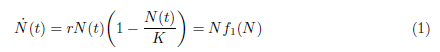
where N(t) denotes the populational density at time 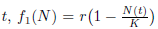 is the per capita population growth rate, r > 0 is the intrinsic growth rate, and K > 0 is the carrying capacity the environment. It is worth observing that in logistic growth, an increment in the population density leads to a negative effect in the reproduction and survival of an individual. On the other hand, the Allee effect means that this negative effect occurs when there is an increment in high densities of populations, whereas in lower densities of populations this increment may be beneficial.
It is widely accepted that the Allee effect may be understood as the cause of the increase in extinction risk at low densities, introducing, in some case, a population threshold that has to be exceeded by population to be able to grow. According with [15], [14], a strong Allee effect introduces a per capita population threshold (the minimal size of the population required to survive), and the population must surpass this threshold to grow (see Figure 1 red line); in contrast, a population with a weak Allee effect does not have a threshold (see Figure 1 green line).
Taking into account the carrying capacity of the environment with respect to the prey in the per capita growth rate of the population, the weak Allee effect has been modeled in [10] by the following differential equation:

in which N(t) denotes the populational density at time 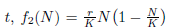 is the per capita population growth rate, 0 < r < 1 is the species growth rate and K > 0 is the carrying capacity of the environment. As mentioned previously, the Allee effect is weak if there exists no critical density population, below which the per capita rate becomes negative. Weak Allee effects are then used to describe cases where the population growth rate is negatively affected by low population sizes, but where the per capita population growth rate cannot go below zero. Therefore populations will grow at low population sizes (see green line in Figure 2).
On the other hand, strong density dependence is used to denote Allee effects where the per capita population growth rate can become negative, which means that there is a critical point in population size below which the population will tend towards extinction (see red line in Figure 2). The strong Allee effect has been modeled in [10] by the following differential equation:
where N(t) denotes the populational density at time 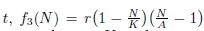 is the per capita population growth rate, r is the species growth rate, K is the carrying capacity, and A is the threshold for the population to not go extinct (0 < A < K).
Based on a widespread evidence in natural populations, several mechanisms have been hypothesized to invoke the Allee effect. Among other phenomena, the most cited and obvious cause of the Allee effect is the difficulty of finding mates at low population sizes in sexually reproducing species. Other mechanisms concern genetic inbreeding, leading to decreased fitness; reproductive facilitation (or cooperative interaction), and predation [15], [14].
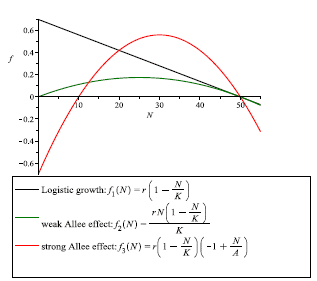
Figure 1
Per capita population growth rate: in the case of logistic growth (black line), we note that the per capita growth rate is a decreasing function of density, an increment in low densities of population leads to a negative effect in the reproduction and survival of an individual; in the case of weak Allee effect (green curve) and strong Allee effect (red curve), we note that unlike to the logistic growth, a negative effect occurs when there is an increment in high densities of populations, whereas in lower densities this increment may be beneficial; the following parameter values r = 0.7, K = 50 and A = 10, were considered for simulations. (For interpretation of the references to color in this figure legend, the reader is referred to the web version of this article).
For all the aforementioned phenomena, and others, the major consequence of the Allee effect is the existence of a critical density below which the aggregation unit considered (that is, population, colony, or social group) is likely to go extinct. The implications of the Allee effect are potentially very important in most areas of ecology and evolution. Particularly, on population dynamics the practical management of population numbers, whether aiming to increase or reduce them, is strongly affected by this effect. The consequences of Allee effects are also significant for the theory of population dynamics, because most classic models imply a linear decrease of growth with density, as opposed to the non-linear relationship associated with the Allee effect.
It is important to observe that the Allee effect has been modeled in different forms [4], [3]. For instance, if in a predator-prey model we assume that the prey growth is damped by the Allee effect and N = N(t) indicates the population size, which depends on time t, the most usual continuous growth equation to express the Allee effect is represented by the following ordinary differential equation:
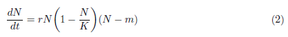
which is the prototypical model for the multiplicative Allee effect. The parameter r in model (2) represents the intrinsic growth rate, K represents the carrying capacity of the environment and m is the Allee effect constant. If -K < m < 0 it shows the weak Allee effect, while if 0 < m < K, it shows the strong Allee effect.
Figure 2
Population growth rate: in the case of logistic growth (black curve), we note that there is no critical point in low densities below which population size is afected, unlike to the weak and strong Allee effects; in the case of weak Allee effect (green curve), we note that the populational growth rate is negatively affected by low population sizes, but where the per capita population growth rate cannot go below zero. Therefore populations will grow at low population sizes; in the case of strong Allee effect (red curve), we note that there is a critical point in population size below which the population will tend towards extinction since for lower population densities, the growth rate is negative; the following parameter values r = 0.7, K = 50 and A = 10, were considered for simulations. (For interpretation of the references to color in this figure legend, the reader is referred to the web version of this article.)
Other mathematical forms have been proposed to describe this phenomenon. Dennis [15] was the first who introduced the equation that modeled the additive Allee effect, represented by the following ordinary differential equation
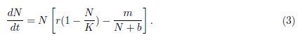
In model (3),  represents the additive term of the Allee effect, m and b are the Allee effect constant with K > b. In absence of predator the prey N has a populational growth given by
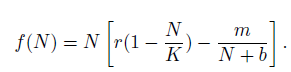
It is clear that f (N) satisfies f (0) = 0 and f'(0) = r - . In the sense of [33], we have the weak Allee effect when m < br, i.e., f '(0) = r -l > 0; the Allee effect will be strong when m > br, i.e., f'(0) = r - < 0. With the previous notation, we conclude that the population presents a weak Allee effect or pure depensation if there exists a value z Є (0,K), such that f ''(z) = 0 and f (N) > 0 for all N Є (0, K) (see Figure 3 green curve). On the other hand, the population presents a strong Allee effect or a critical compensation if for lower population densities, the growth rate is negative, that is, for small values of N near to zero, we have f(N) < 0 (see Figure 3 red curve). When the species is submitted to a strong Allee effect, it may have a bigger tendency to be less able to overcome these additional mortality causes, to have a slower recovery, and to be prone to extinction than other species [28]. These curves are called decompensation curves, and there exist a value of z Є (0,K), such that f (z) = 0. The value of N = z is an unstable equilibrium and coincides with m in the equation for the multiplicative Allee effect, which is called the minimal level of viable population or threshold level. If the initial population N0 at time t = 0 is less than m, i.e., N(0) = N0< m, then for this initial size of population less than m the population tends to extinction.
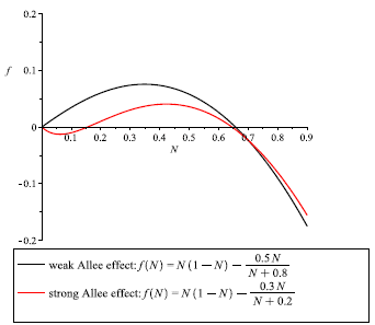
Figure 3
Graphics for the function f (N) = N(1 - N) -mNN+b in the cases: Weak Allee effect m < br (green curve): r = 1, K =1, m = 0.5, b = 0.8; Strong Allee effect m > br (red curve): r = 1, K = 1, m = 0.3, b = 0.2. (For interpretation of the references to color in this figure legend, the reader is referred to the web version of this article.)
In recent studies [23], [15], [11], [20], [13], the authors studied the spatio-temporal dynamics for a predator-prey model with diffusion and Allee effect. In [4], [3] the existence and stability of limit cycles for a Leslie-Gower predator prey model with additive Allee effect was studied. In [13] the authors analyzed a predator-prey model with diffusion and Holling type II functional response subject to additive Allee effect in the prey equation.
Following [13], we focus our attention on the following system of equations:
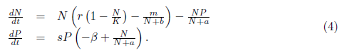
The parameters composing the model (4) are positive, and r, K, m, b have the same meaning as in Equations (2) and (3); a is a saturation constant; ß is the death rate of the predator; and s is the feed concentration; Dennis [15] showed that the probability of mating encounters among individual of a population with increasing population density, could be modeled using a rectangular hyperbola function , where b is the population size at which mating fitness is half of its maximum value that is, b is the population density at which the probability of mating is . Therefore, 1 - = the probability of not mating. Consequently, the term - considered in the per capita growth rate of prey population in model (4) represents the reduction due to mating shortage. We then have the logistic model adjusted for mating encounters. - is the predation rate where the saturation constant a reflects the prey density level at which the predation rate begins to saturate, meaning that predators have a limited capacity to consume prey and this capacity stabilizes at high prey densities; is the fraction of the maximum consumption rate of prey by predators as a function of prey density.
In [13] the authors investigated the dynamics of model (4) and its diffusive version. They analysed the local and global asymptotic stability behavior of the positive equilibrium for both the ODE system and the reaction diffusion system. Furthermore, they obtained conditions over the parameters for the occurrence of the Hopf bifurcation in model (4) in the cases of weak Allee effect as well as strong Allee effect. However, to the best of our knowledge there is no results related to the direction and stability of the bifurcating periodic orbits for the system (4). In this paper, we determine the direction and stability of the bifurcating periodic orbits for the system, in the case of weak Allee effect as well as strong Allee effect by calculating the value of the first Lyapunov coefficient.
This paper is organized as follows: In Section 2 we present a review of the method found in [26] for the calculation of the first Lyapunov coefficient for a general ordinary differential equation system. In Section 3, positivity, dissipation, boundedness and permanence of the solutions for model (4) are studied. In Section 4, equilibrium points of the system (4) are identified, and a Hopf bifurcation analysis for the positive equilibrium is carried out. We determine the direction and stability of the bifurcating periodic orbits for the system (4), in the case of weak Allee effect as well as strong Allee effect by calculating the value of the first Lyapunov coefficient; simulations are presented to corroborate the analytical results. Also, in the case of strong Allee effect it is observed by a numerical experiment the presence of an interesting global bifurcation not discussed earlier for this mode. A discussion follows in the final section.
2. Outline of the Hopf Bifurcation Methods
In this section we present a very brief summary of the projection method described in [26] for the calculation of the first Lyapunov coefficient associated with the Hopf bifurcation, denoted by l1. Other equivalent definitions and algorithmic procedures to write the expressions of the Lyapunov coefficients for two-dimensional systems can be found in [7] and [27], among others.
Definition 2.1. Consider the differential equation
where X ∈ ℝ 2 is a vector representing phase variables and m ∈ ℝ is a parameter representing control parameter. Assume that f is of class C∞ in R2× ℝ. Suppose that system (5) has an equilibrium point X = X0, which may depend on m. Let the eigenvalues of the linearised system about this equilibrium point be given by λ1,2 (m) = α(m) ± iω(m), and suppose that this pair of simple complex eigenvalues reaches the imaginary axis as the parameter m varies, say at a critical value m = m∗ , and we have λ1,2 (m∗ ) = ±iω0, ω0> 0. The bifurcation corresponding to the presence of λ1,2 (m∗ ) = ±iω0, ω0> 0, is called a Hopf (or Andronov-Hopf) bifurcation. Specifically, at the bifurcation point, a complex conjugate pair of eigenvalues crosses the imaginary axis of the complex plane, leading to the creation or destruction of a periodic orbit.
Now, consider the system (5) and suppose that it has an equilibrium point X = X0 at m = m* and, denoting the variable X - X0 also by X, we write
Where
with J = fX (0, m∗ ) and B(X, Y ), C(X, Y, Z) are multilinear functions. In coordinates, we have
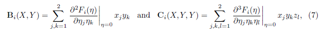
where i = 1, 2.
Suppose that (0, m∗ ) is an equilibrium point of (5) where the Jacobian matrix J has a pair of pure imaginary eigenvalues λ1,2 = ±iω0, ω0> 0, and these eigenvalues are the only pure imaginary eigenvalues. Let Tc be the generalized eigenspace of J corresponding to λ1,2 . By this it is meant the largest subspace invariant by J on which the eigenvalues are λ1,2
Let p, q ∈ C2 be complex eigenvectors corresponding to −iω0 and +iω0 respectively, such that
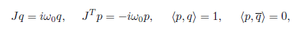
where JT is the transpose of the matrix J and  is the standard scalar product in ℂ2 (linear with respect to the second argument). Thus, the critical real eigenspace Tc corresponding to ±iω0 is now two-dimensional, and is spanned by {Req, Imq} and any vector Y ∈ Tc can be represented as Y = wq + w¯q¯, where w = p, Y ∈ ℂ.
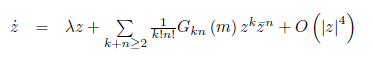
By introducing a complex variable z, system (5) can be written for sufficiently small |m| as a single equation:
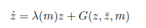
where G = O(|z4I|) is a smooth function of (z, , m) and
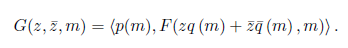
Write G as a formal Taylor series in two complex variables (z and ,):
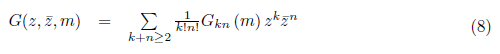
Where
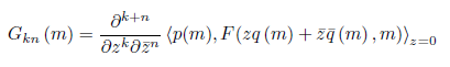
for k + n > 2.
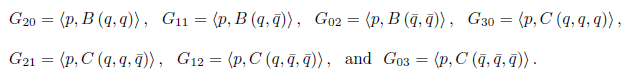
On the other hand
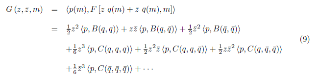
comparing (8) with (9), we have
Also, the equations
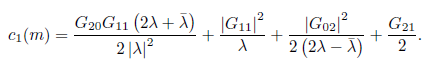
where λ = λ (m) = α (m) ± iω (m) , α (m∗ ) = 0, ω (m∗ ) = ω0> 0 can be transformed by an invertible parameter- dependent change of complex coordinate, for all sufficiently small |m| , into an equation with only the resonant cubic term:
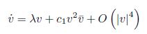
where c1= c1(m) and
At the bifurcation parameter value m = m*, the previous equation reduces to
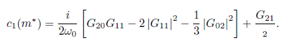
From Lemma 3.7 pp. 98 of [26], the equation
where α (m∗ ) = 0, ω (m∗ ) > 0 and supposing that α′ (m∗ ) # 0, and Re(c1(m∗ )) # 0, then, the equation can be transformed by a parameter-dependent linear coordinate transformation, a time rescaling, and a nonlinear time reparametrization into an equation of the form
where u is a new complex coordinate, and θ, β are the new time and parameter, respectively,
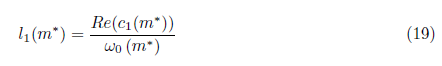
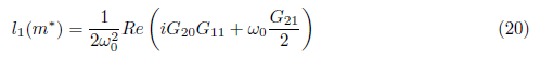
Definition 2.2. The real function l1() is called the first Lyapunov coefficient. It follows from (19) that the first Lyapunov coefficient at = 0 can be computed by the formula

Proposition 2.3. Consider system (5) where X Є ℝ 2is a vector representing phase variables and m Є ℝ is a parameter representing control parameter. Assume that f is of class ℂ∞in ℝ2x ℝ. Suppose that (5) has an equilibrium point X = X0 at m = m*. Then the following holds:
-
Suppose that at (X0, m∗ ) the Jacobian matrix A of (5) has a pair of pure imaginary eigenvalues λ2,3 (m∗ ) = ±iω0, ω > 0, and these eigenvalues are the only eigenvalues with null real part. Then (X0, m∗ ) is a Hopf point of (5).
-
At (X0, m∗ ) a two-dimensional center manifold is well-defined, it is invariant under the flow generated by (5) and can be continued with arbitrary high class of differentiability to nearby parameter values.
-
If Reλ(m)|m=m∗ # 0 then (X0, m∗ ) is a transversal Hopf point. In this case, if l1 # 0 then the system (5) undergoes a Andronov-Hopf bifurcation, that is, in a neigh-borhood of (X0, m∗ ) the dynamic behavior of the system (5), reduced to the family of parameter-dependent continuations of the center manifold, is orbitally topologically equiv-alent to the following complex normal form
where w ∈ ℂ, η, ω and l1are real functions having derivatives of arbitrarily higher order, which are continuations of 0, ω0and the first Lyapunov coefficient at the Hopf point. When l1(m∗ ) < 0 (resp. l1(m∗ ) > 0) a family of stable (resp. unstable) periodic orbits can be found in these manifolds, shrinking to an equilibrium point at the Hopf point.
iv) The Hopf bifurcation is supercritical (resp. subcritical) if Reλ(m)|m=m∗)−1l1(m∗) < 0 (resp. > 0). In addition, the bifurcating periodicsolutions are stable (resp. unstable) if l1(m∗) < 0 (resp. l1(m∗) > 0).
3. Positivity, dissipation, boundedness and permanence of the solutions
In this section, we are mainly concerned with some simple properties of the solution to model (4). In theoretical ecology, positivity and boundedness of the system establishes the biological well behaved nature of the system. On the other hand, persistence and permanence are important in the sense that they describe long term behavior of the system. Due to many reasons, for example, pollution, over predation, over exploitation, mismanagement of natural resources, among others, several species become extinct and many others are at the bound of extinction. Accordingly, the concept of persistence, that means the survival of species for a longer time, has drawn lot of attention (see [9], [21],[1], [2]).
Analytically, a system is said to be persistent if it persist for each population, that is, if lim inft→∞x(t) > 0 (stronger case) or lim supt→∞x(t) > 0 (weaker case) for each population x(t) of the system. Geometrically, persistence means that trajectories that initiate in a positive cone are eventually bounded away from coordinate planes. On the other hand permanently coexistence (uniform persistence) implies the existence of a region in the phase space at a non zero distance from boundary, in which all the population vectors must ultimately lie. The later one assures the survival of species in biological sense.
It is worth observing that in many significant examples of periodic differential systems modeling infectious diseases transmission, competition of species among others ecological models, it is of interest to prove the existence of a nontrivial fixed point for the operator associated with the differential system, which establishes the global existence of nontrivial periodic solution that may implies the coexistence of the species. To this end, some well known theorems or techniques can be applied such as Browder theorem [12], Brouwer degree techniques, Leray-Schauder degree techniques if the space of initial values is infinite dimensional, among others.
Although the phenomenons such as periodicity of a differential systems, uniform persistence, existence of a compact global attractor with some more conditions, often implies the global existence of a positive fixed point for the system, the focus of our paper is to study the existence of periodic orbits for the non-periodic system (4) by Hopf bifurcation arguments, which are local existence results. Nevertheless, for sake of completeness, results concerning the persistence and permanence of system (4) are presented in this section, since those results guarantee the the survival of the total population which is desirable on the study of population dynamics. Mathematically, persistence of a system means that strictly positive solutions do not have any omega limit points on the boundary of the positive cone.
We highlight that the study of system (4) involving periodic cases to obtain some sufficient conditions on the boundedness, permanence, extinction and global existence of a positive fixed point will be considered in a next exposition, since our focus here is carrie out a local analysis by Hopf bifurcation arguments.
Definition 3.1. The system system (4) is said to be weakly persistent if every solution (N(t), P(t)) satisfies two conditions:
-
N(t) ≥ 0, P (t) ≥ 0, for all t ≥ 0.
-
lim supt→∞N(t) > 0, lim supt→∞P (t) > 0.
System (4) is said to be strongly persistent if every solution (N(t),P(t)) satisfies the following condition along with the first condition of the weak persistence:
lim inft→∞N(t) > 0, lim inft→∞P (t) > 0.
Remark 3.2. Weak persistence allows that liminft→∞N(t) =0 or liminft t→∞P(t) = 0 so that arbitrarily small statistical fluctuations may annihilate a species [24].
Definition 3.3. The system (4) is said to be permanent if there exist positive constants s and S, with 0 < s < S such that
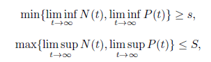
for all solutions (N(t), P(t)) of system (4) with positive initial values. System (4) is said to be non-permanent if it has a positive solution (N(t), P(t)) such that min{liminft→∞N(t), lim inft→∞P(t)} = 0.
The following results ensure the positivity, boundedness, dissipativeness and permanence of solutions of system (4).
Lemma 3.4. The positive quadrant of ℝ 2+is invariant for the system (4).
Proof. The first quadrant is an invariant region for (4) since {(N,P) G ℝ 2+: N = 0} and {(N,P) G ℝ 2+: P = 0} are invariant manifolds of (4). Therefore, the solutions of (4) with the initial values N(0) > 0 and P(0) > 0 are positive. The basic existence and uniqueness theorem for differential equations ensures that positive solutions and the axis cannot intersect. 0
Theorem 3.5. The system (4) is dissipative when t > 0 and N(to),P((to) > 0.
Proof. From the first equation of system (4), we have 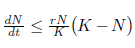 . By integrating the previous inequality from to to t, it follows that
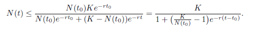
Letting t → ∞ in the previous inequality, it follows that lim sup→ ∞N (t) ≤ K. As a consequence, for any ϵ1> 0,, there exists a T1> 0 such that N ≤ K + ϵ1 for t > T1..
On the other hand, multiplying the first equation in (4) by s and then adding with the second one, we obtain (sN + P )′ ≤ srN − sβP. Let ξ = maxt≥0{srN(t) + s2βN(t)}. Then we have sN +P _′ ≤ ξ −sβ(sN +P). From Gronwall’s inequality, we obtain that
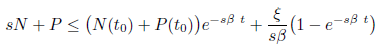
as long as the solution exists. Letting t → ∞ in the previous inequality, it follows that lim supt→∞ (sN + P ) ≤ . Hence P (t) is also bounded. As a consequence, for any ϵ2> 0, there exists a T2> 0 such that sN + P ≤ + ϵ2 for t > T2. This completes the proof of the boundedness of solutions and the system under consideration is weakly persistent (dissipative). Hence, any solution is defined for t > 0 and enter the attracting compact set
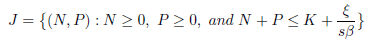
for sufficiently large values of t, which implies that J is positive invariant. Consequently, the system is dissipative and its global attractor is contained in J. 0
Remark 3.6. We observe that in the case of m = 0, i.e., in model (4) without Allee effect, the dissipation and boundedness of the solution are similar to the results in Theorem 3.5. In other words, the solutions of the system without Allee effect are always dissipative and uniformly bounded.
Theorem 3.7. If m > rb - holds, then any solution of system (4) starting from the interior of the first quadrant satisfies lim inft→∞N(t) ≥ 0, lim inft→∞P(t) ≥ 0.
Proof. From Theorem 3.5 it is clear that N(t) ≤ K + ϵ1 and P(t) ≤ + ϵ2 for t ≥ T = max{T1,T2}. Therefore, from the first equation of system (4) we have

for t ≥ T. Thus, using a comparison theorem (see [8] pp. 1071) and the arbitrariness of ϵ2 > 0, we obtain liminft→∞N(t) ≥ 0 provided K - < 0 or equivalently m > rb - . On the other hand, observe that P' ≥ -ßP, hence lim inft→∞P(t) ≥ 0.
Remark 3.8. According with Theorem 3.7, we may have lim inft→∞N(t) = lim inft→∞P(t) = 0, provided m > rb - . This condition implies that the system is non-permanent. Such a scenario occur when the system (4) is weakly persistent, allowing arbitrarily small statistical fluctuations to lead to the extinction of a species. This annihilating phenomenon may take place when the system (4) is subject to strong Allee effect, i.e., m > rb. Clearly this inequality highlights the contribution of the strong Allee effect.
4. Equilibria, stability and Hopf bifurcation
In this section, equilibrium points of the system (4) are identified and a Hopf bifurcation analysis for the positive equilibrium is carried out. It is worth noting that in [13], assuming a < b in case of weak Allee effect and a = b in case of strong Allee effect, the authors proved that the model (4) undergoes a Hopf bifurcation around its positive equilibrium at
Even though they have focused on the study of Hopf bifurcation for the system (4), there is no result concerning the direction of the Hopf bifurcation and stability of the bifurcating periodic solutions. Our main goal in this section is to determine the direction of the Hopf bifurcation and the stability of the bifurcating periodic solutions for this system, when additive Allee effect is considered in the prey equation. First, we focuses on the case when the Allee effect in (4) is the weak one, i.e., m < br. Next, we analyze the system (4) when the Allee effect is the strong one, i.e., m > br.
It was observed in [25] that because of difficulties in finding mates when prey population density becomes low due to increasing emigration rate, Allee effect may occur in prey species. These two mechanisms are related, because high rates of emigration further decrease density, thereby reducing the probability of locating mates at low densities. Consequently, these two mechanism may increase the risk of extinction of small local population. As we will see in this section, the predator-prey model with weak Allee effect may not increase the extinction risk of both predators and prey. However, when the model is subject to strong Allee effect it may increase the extinction risk of both species.
4.1. The case of weak Allee effect
Let us assume m < br. As a starting point of this subsection, we discuss the equilibria of system (4) that is, the solutions of the system
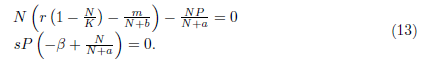
Following the ideas in [13], one can verify that model (4) has always two boundary equilibria
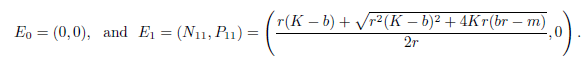
On the other hand, system (4) has a unique positive equilibrium E* = (N*, P*) provided
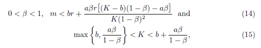
where
In this subsection, we will assume the conditions given in (14) from now on.
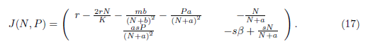
The Jacobian matrix associated with the system (4) is given by
The authors in [13] observed that the equilibria E0 and Ei are saddle point for model (4).
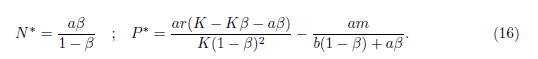
Remark 4.1. When the system (4) is compared with the predator prey model without Allee effect, whose boundary equilibria E0= (0, 0) and Er= (Nj, 0) are also saddle points, we can see that if the Allee effect of the prey population in system (4) is very weak, it may not increase the extinction risk of both predators and prey. However, when model (4) is subject to a strong Allee effect it may not be true as we will see in the next subsection. Furthermore, since the positive equilibrium of model (4) without Allee effect is given by 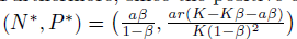 , provided K >
 and ß < 1, this is obvious from (16) that the equilibrium density of prey population is the same, however, the equilibrium density of predator population is smaller. That is, a decrease of predator population density at the equilibrium is caused by the Allee effect of prey population. This highlights the extinction risk caused by the Allee effect.
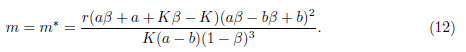
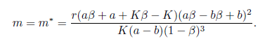
In the following, we collect the main results given in [13] related to the stability of the equilibrium E*, with few modifications which guarantee the positivity of m*.
Theorem 4.2. (i) If K(1 - ß)3(α - b)m < r(Kß - K + α + α ß)( α ß + b - bß)2holds, then the equilibrium point E* is locally asymptotically stable for the system (4) .
(ii) If K(1 -ß)3(α - b)m > r(Kß - K + α + α ß)( α ß + b - bß)2point E* is unstable for the system (4).holds, then the equilibrium
(iii) Assume that a < b and aß + a + Kß - K < 0. Then the system (4) undergoes a Hopfbifurcation around the positive equilibrium E*at
(iv) Assume that a <b, rb2(K - a) < K (b - a) m and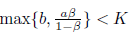 < min{a + b,b + } holds. Then E * is globally asymptotically stable for the system (4).
The Jacobian matrix of model (4) evaluated at E*= (N*, P*) takes the form
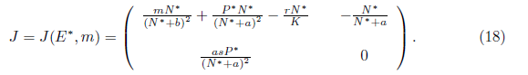
It is easy to see that 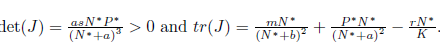
In the next theorem we determine the direction of the Hopf bifurcation and stability of the bifurcating periodic solutions for the system (4) To this purpose, we follow the frame work of Section 2 (see also [35], [19] and [26]). We highlight that these results were not established in [13]
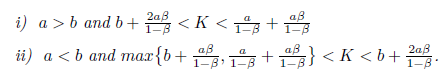
Theorem 4.3. Assume that one of the following two conditions is true:
-
a <b and aß + a + Kß - K < 0;
-
a > b and aß + a + Kß - K > 0.
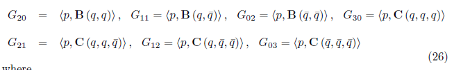
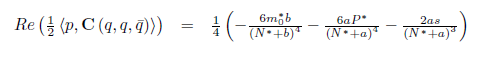
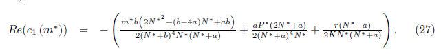
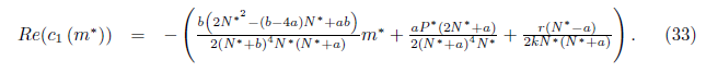
Then the system (4) undergoes a Hopf bifurcation around the positive equilibrium E*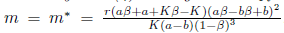 . Furthermore, the first Lyapunov coefficient associated with the equilibrium E*is given by
or equivalently
with
where

If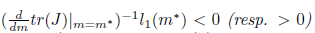 the Hopf bifurcation is supercritical (resp. subcritical) for the system (4). On the other hand, if l1(m*) < 0 (resp. > 0) the bifurcating periodic solutions are stable (resp. unstable).
Proof. To determine the direction of the Hopf bifurcation, we will calculate the first Lyapunov coefficient for the system (4) at m = m*. Note that E* = (N*,P*) is the unique positive equilibrium of system (4) and the Jacobian matrix of system (4) evaluated at (E*,m*) is given by
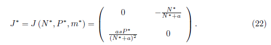
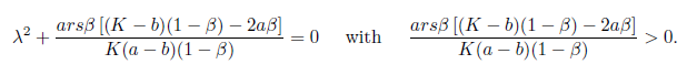
The Jacobian matrix (22) has the purely imaginary eigenvalues
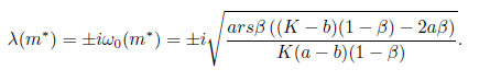
From [13] we have
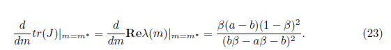
Note that the characteristic equation associated with the matrix given in (22) is (23)
The eigenvectors associated with the eigenvalues 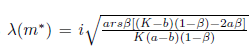 and
and 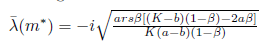 are, respectively,
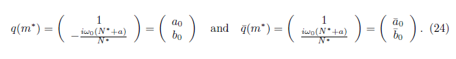
On the other hand, the transposed matrix of J is given by
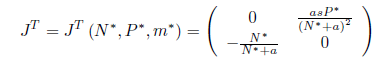
where

Are the eigenvectors of JT associated with the eigenvalues λ(m*) =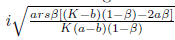 and
and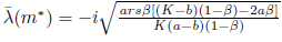 respectively.
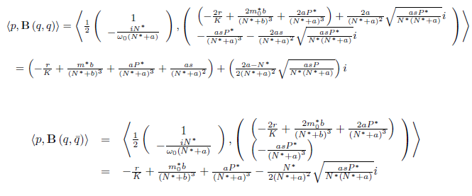
We calculate the terms  and
and  given in Section 2 which are evaluated at (E*, m*). Given that
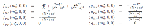
we have
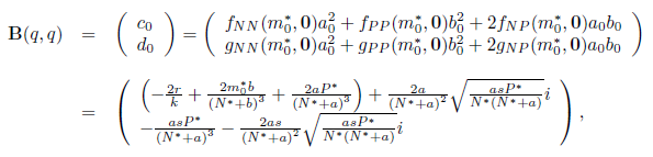
and
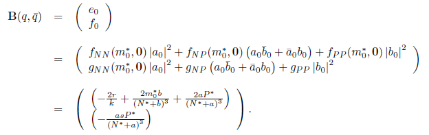
On the other hand, since
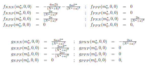
we have
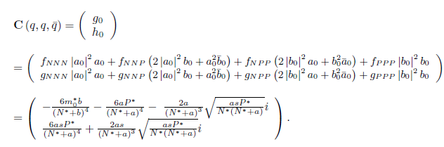
For the sake of convenience we denote q(m*) as q and p(m*) as p, as well as its conjugates. On the other hand, we get
Where
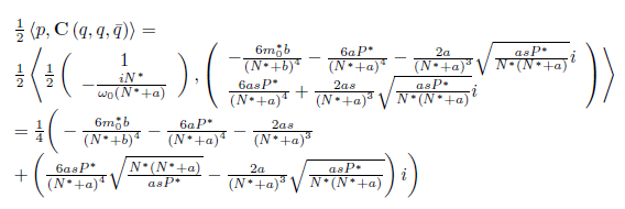
therefore,
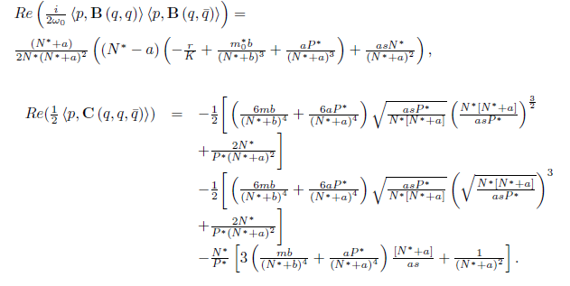
and
finally,
Consequently, according with [26] and taking into account (23) if a < b, aβ + a + Kβ - K< 0, and l1(m∗ ) > 0 (resp. l1(m∗ ) < 0), the Hopf bifurcation is supercritical (resp. subcritical) for the system (4), and the bifurcating periodic solutions are unstable (resp. stable). On the other hand, if a > b, aβ + a + Kβ − K > 0 and l1(m∗ ) < 0 (resp. l1(m∗ ) > 0), the Hopf bifurcation is subcritical (resp. supercritical) for the system (4) and the bifurcating periodic solutions are stable (resp. unstable).
Remark 4.4. It is worth highlighting that the results obtained in Theorems 4 and 5 concerning the existence of periodic orbits for the non-periodic system (4), are local results which were obtained by Hopf bifurcation arguments. As observed in Section 3, the analysis of system (4) involving periodic cases, will be considered in a next exposition since our main purpose in this paper is to carrie out a local stability and bifurcation analysis for the proposed system.
In the following propositions we give conditions on the parameters such that the expression (21) becomes negative, which implies that lp(m*) < 0 and consequently, the bifurcating periodic orbits of system (4) around the equilibrium E* are stable.
Remark 4.5. It is clear that φ(N∗ ) = 2N∗2− (b − 4a) N∗ + ab is a quadratic function, which geometrically represents a parabola that opens upwards and whose vertex is given by the point  which is positive as long as the discriminant of the equation φ(N∗) = 0 is negative or equivalent when 16ab > b2 + 16a2. Consequently φ(N∗) > 0, if 16ab > b2 + 16a2.
Taking into account Remark 4.5, we can establish the following propositions.
Proposition 4.6. If m b2 + 16a2and
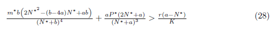
then l1(m*) < 0. Moreover, if . Consequently, the system (4) undergoes a subcritical Hopf bifurcation arround the equilibrium point E* at
Furthermore, according with Theorem 3.3 page 100 in [35], the bifurcating periodic solutions are stable.
Proof. It is clear that the conditions 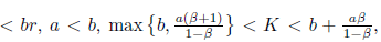
 and (28) imply that m* > 0, P* > 0, ω0(m*) > 0 and hence l1(m*) =
 . Furthermore, by (23) we have
  .
.
The Figure 4 illustrates the result obtained in Proposition 4.6.
Proposition 4.7. If m and
and
then l1(m*) < 0. Moreover, if α > b we have . Consequently, the system (4) undergoes a supercritical Hopf bifurcation arround the equilibrium point E*at
![Subcritical Hopf bifurcation around the positive equilibrium (0.157, 0.085). The simulations were carried using MATCONT [16] to illustrate the result obtained in Proposition 4.6, by choosing the values of parameters: (a) a = 0.1, b = 0.7, ß = 0.6, K = 0.71, r =1, s = 0.1, m = 0.52, (N*,P*) = (0.15,0.043). (b) a = 0.1, b = 0.7, ß = 0.6, K = 0.71, r =1, s = 0.1, m* = 0.516, (N*,P*) = (0.15,0.0446). (c) a = 0.1, b = 0.7, ß = 0.6, K = 0.71, r = 1, s = 0.1, m = 0.5, (N *,P *) = (0.15,0.049).](../2145-8472-rein-42-02-23-gf4.png)
Figure 4
Subcritical Hopf bifurcation around the positive equilibrium (0.157, 0.085). The simulations were carried using MATCONT [16] to illustrate the result obtained in Proposition 4.6, by choosing the values of parameters: (a) a = 0.1, b = 0.7, ß = 0.6, K = 0.71, r =1, s = 0.1, m = 0.52, (N*,P*) = (0.15,0.043). (b) a = 0.1, b = 0.7, ß = 0.6, K = 0.71, r =1, s = 0.1, m* = 0.516, (N*,P*) = (0.15,0.0446). (c) a = 0.1, b = 0.7, ß = 0.6, K = 0.71, r = 1, s = 0.1, m = 0.5, (N *,P *) = (0.15,0.049).
Furthermore, according with Theorem 3.3 page 100 in [26], the bifurcating periodic solutions are stable.
Proof. It is clear that the conditions  b2+ 16a2 and (29) imply that m* > 0, P* > 0, ω0(m*) > 0 and hence l1(m*) =
 . Furthermore, by (23) we
  .
.
The Figure 5 illustrates the result obtained in Proposition 4.7.
4.2. The case of strong Allee effect
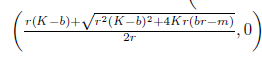
Following the ideas in [13], assume that m > br, that is, the Allee effect in model (4) is strong. One can verify that model (4) has one boundary equilibrium E0= (0,0). If  the system (4) has other two boundary equilibria
 .
.
![Supercritical Hopf bifurcation around the positive aquilibrium (0.2,0.5). The simulations were carried using MATCONT [16] to illustrate the result obtained in Proposition 4.7, by choosing the values of parameters: (a) a = 0.7, b = 0.2, ß = 13, K = 1, r =1, s = 0.2, m = 0,14, (N*,P*) = (0.3, 0.42). (b) a = 0.7, b = 0.2, ß = 3, K =1, r = 1, s = 0.2, m* = 0, 15, (N * ,P *) = (0.3,0.4). (c) a = 0.7, b = 0.2, ß = 1, K =1, r = 1, s = 0.2, m = 0, 16, (N*,P*) = (0.3, 0.38).](../2145-8472-rein-42-02-23-gf5.png)
Figure 5
Supercritical Hopf bifurcation around the positive aquilibrium (0.2,0.5). The simulations were carried using MATCONT [16] to illustrate the result obtained in Proposition 4.7, by choosing the values of parameters: (a) a = 0.7, b = 0.2, ß = 13, K = 1, r =1, s = 0.2, m = 0,14, (N*,P*) = (0.3, 0.42). (b) a = 0.7, b = 0.2, ß = 3, K =1, r = 1, s = 0.2, m* = 0, 15, (N * ,P *) = (0.3,0.4). (c) a = 0.7, b = 0.2, ß = 1, K =1, r = 1, s = 0.2, m = 0, 16, (N*,P*) = (0.3, 0.38).
It is not difficult to determine that the equilibria E0 is always locally stable, E1 and E2 are saddle points.
Finally, if

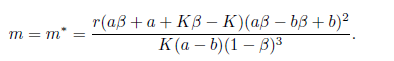
holds, then the system (4) has a unique positive equilibrium E*= (N*, P*) where 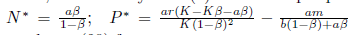 . In this subsection, we will assume the condition (30) from now on.
In the following theorem, we summarize the main result from [13] regarding the stability of the equilibrium point E* under the influence of a strong Allee effect, with a few adjustments ensuring the positivity of m* .
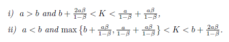
Theorem 4.8. Assume that one of the following conditions are true:
Then:
- 1. (1) If K(1 − β)3(a − b)m < r(Kβ − K + a + aβ)(aβ + b − bβ)2holds, the equilibrium point E∗is locally asymptotically stable for system (4).
- 2. If K(1 − β)3(a − b)m > r(Kβ − K + a + aβ)(aβ + b − bβ)2holds, the equilibrium point E∗is unstable for system (4).
- 3. The system (4) undergoes a Andronov-Hopf bifurcation at
We prove in the next theorem that if model (4) does not have neither boundary equilibria nor interior equilibrium, i.e., if the Allee effect of prey population is very strong, then E0 is globally asymptotically stable. Any positive orbit converges to E0 as t tends to infinity, meaning prey and predators cannot coexist even if the initial population density of prey is abundant. As observed in Remark 3.8, this annihilating phenomenon of the species may occur due to the weakly persistence of system (4) subject to strong Allee effect. A typical phase portrait is shown in Figure 6.
Theorem 4.9. Let cp and C2 be positive constants. The equilibrium point Eo of system (4) is globally asymptotically stable provided cp > C2S and m > r(b + K). In this case, the only equilibrium point ofsystem (4) iso.
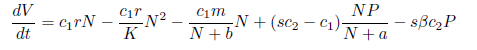
Proof. Consider the following Lyapunov function V(N, P) : ℝ2+- ℝ defined by V(N(t), P(t)) = cpN(t) + c2P(t). The time derivative of V along the solutions of system (4) is
Taking into account that limt→∞N(t) ≤ K, we have, for t→ ∞ , that
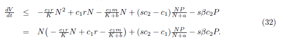
Now, 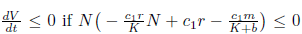 and sc2- cp< 0. The last inequality is equivalent to c1> sc2. On the other hand, define
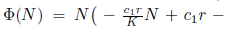
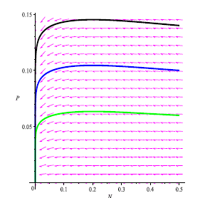
Figure 6
We made the phase portrait using MAPLE 13 to illustrate the global stability of Eo = (0,0) by choosing: a = 0.6; b = 0.6; ß = 0.25; K =1; r =1; m = 0.7; s = 0.1. Here, m and
 which is a parabola with concavity towards down, whose zeros are N1* = 0 and
 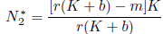 . Thus, if N2 < 0 we have Φ(N) ≤ 0 for all N ≥ 0. This is the case if m ≥ r(K + b). Finally, observe that:
i) 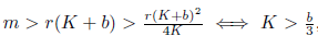 , which is true since K > b. This implies that system (4) has no boundary equilibria other than E0.
ii) 
 > 0. If we define
 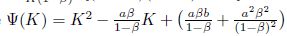 , we easily conclude that ty(K) > 0 for all K > 0 since the the parabola has concavity towards up and its zeros are complex conjugate. Consequently, this implies that system (4) has no positive equilibria within ℝ2+. 0
Remark 4.10. In model (4) without a strong Allee effect, the boundary equilibria are E0 = (0,0) and Ef = (Nf, 0) both of which are saddle points. There exists a positive equilibrium E*, feasible under conditionsd  and ß < l. The equilibrium E0 of system (4) is always a locally stable node, implying that both prey and predators will become extinct if their population densities enter the attraction region of E0. In particular, if the population density of prey becomes less than
  , then both predators and prey will go extinct (A typical phase portrait is shown in Figure 7). It is important to observe that the unstable manifold of the equilibrium E2 goes toward the interior equilibrium (blue curve in Figure 7), and the stable manifold of Ef (black curve in Figure 7) is above the unstable manifold of E2. The model (4) when compared with the predator-prey model without Allee effect, increases the extinction risk of both predators and prey due to the presence of strong Allee effect in the prey population.
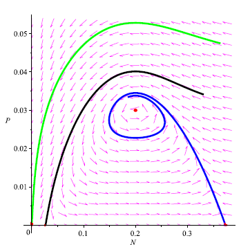
Figure 7
We made the phase portrait using MAPLE 13 to illustrate that prey and predators will become extinct when their population densities lie in the attraction region of Eo by choosing: a = 0.6; b = 0.6; ß = 0.25; K =1; r = 1; m = 0.61; s = 0.1. The critical points on the plane N P are points: E0 = (0,0), E1 = (0.02679491925, 0), E2 = (0.3732050808,0) and E* = (0.2, 0.03).
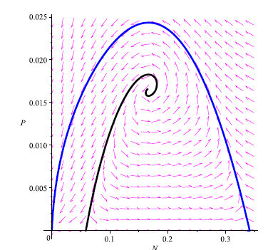
Figure 8
We made the phase portrait using MAPLE 13 to illustrate that prey and predators will become extinct when their population densities lie in the attraction region of Eo. However, if we take initial conditions on the stable manifold of E1 (black curve) it means the coexistence of the prey population. We choose the parameter values: a = 0.5; b = 0.6; ß = 0.25; K = 1; r = 1; m = 0.62; s = 0.1. The critical points on the plane N P are points: Eo = (0,0), E1 = (0.02679491925,0), E2 = (0.3732050808, 0) and E* = (0.2, 0.03).
Remark 4.11. It is worth observing that in Figure 7 the stable manifold of the equilibrium point E1 is above the unstable manifold of the equilibrium point E2. On the other hand, in Figure 8 the stable manifold of the equilibrium point Ei is below the unstable manifold of the equilibrium point E2. This suggests that heteroclinic cycles occurs in model (4) for certain values of the parameters. This numerical experiment confirms the presence of an interesting global bifurcation not discussed earlier for this model. Accordingly we have the following:
Conjecture In view of remark 4.11, we conjecture that heteroclinic cycles occurs in model (4) for certain values of the parameters.
In the following, we determine the direction of the Hopf bifurcation and the stability of the bifurcating periodic solutions in the case of strong Allee effect for the system (4).
Theorem 4.12. Assume that one of the following two conditions is true:
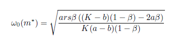
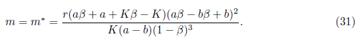
Then, the system (4) undergoes a Hopf Bifurcation around the positive equilibrium E* = (N*, P*) at m = m* given by (31). Furthermore, the first Lyapunov coefficient associated with the equilibrium E* is given by (19), where
If  the Hopf bifurcation is supercritical (resp. subcritical) for the system (4). On the other hand, if l1(m*) < 0 (resp. > 0) the bifurcating periodic solutions are stable (resp. unstable).
Proof. The proof is analogous to that given in Theorem 4.3 and therefore will be omitted.
In the following propositions, taking into account Remark 4.5, we give conditions on the parameters such that the expression (33) becomes negative, which implies that li (m*) < 0 and consequently the bifurcating periodic orbits of system (4) around the equilibrium E* are stable.
Proposition 4.13. If br 
 , and
, and
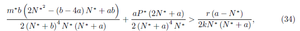
then l1 (m*) < 0. Moreover, if a < b we have -  . Consequently, the system (4) undergoes a subcritical Hopfbifurcation around the equilibrium point E* at
Furthermore, the bifurcating periodic solutions are stable.
Proof. The conditions 
 and (34) imply that N * > 0, P * > 0, m* > 0 and hence l1 (m*) < 0. Furthermore, by (23) we have
  < 0 if a <b. 0
The Figure 9 illustrates the result obtained in Proposition 4.13.
![Subcritical Hopf bifurcation around the positive equilibrium (0.3,0.22). The simulations were carried using MATCONT [16] to illustrate the result given by Proposition 4.13, by choosing the values of parameters: (a) a = 0.1, b = 0.3, ß = 0.5, K = 0.49, r = 0.2, s = 0.1, m = 0.061, (N*,P*) = (0.1,0.0013). (b) a = 0.1, b = 0.3, ß = 0.5, K = 0.49, r = 0.2, s = 0.1, m* = 0.062, (N*,P*) = (0.1, 0.00083). (c) a = 0.1, b = 0.3, ß = 0.5, K = 0.49, r = 0.2, s = 0.1, m = 0.063, (N*,P*) = (0.1, 0.00033).](../2145-8472-rein-42-02-23-gf9.png)
Figure 9
Subcritical Hopf bifurcation around the positive equilibrium (0.3,0.22). The simulations were carried using MATCONT [16] to illustrate the result given by Proposition 4.13, by choosing the values of parameters: (a) a = 0.1, b = 0.3, ß = 0.5, K = 0.49, r = 0.2, s = 0.1, m = 0.061, (N*,P*) = (0.1,0.0013). (b) a = 0.1, b = 0.3, ß = 0.5, K = 0.49, r = 0.2, s = 0.1, m* = 0.062, (N*,P*) = (0.1, 0.00083). (c) a = 0.1, b = 0.3, ß = 0.5, K = 0.49, r = 0.2, s = 0.1, m = 0.063, (N*,P*) = (0.1, 0.00033).
Proposition 4.14. If br
 and
and
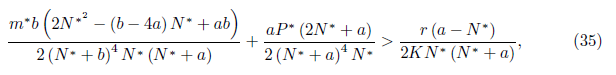
then l1(m*) < 0. Moreover, if a > b we have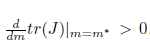 . Consequently, the system (4) undergoes a supercritical Hopf bifurcation around the equilibrium point E* at
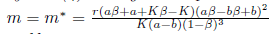 . Furthermore, the bifurcating periodic solutions are stable.
Proof. The conditions  α> b, 16ab > b2+ 16a2, and (35), imply that N * > 0, P * > 0, m* > 0, and l1(m*) < 0. Furthermore, by (23) we
  .
.
The Figure 10 illustrates the result obtained in Proposition 4.
![Supercritical Hopf bifurcation around the positive equilibrium (0.3, 0.22). The simulations were carried using MATCONT [16] to illustrate the result given by Proposition 4.14, by choosing the values of parameters: (a) a = 0.8, b = 0.45, ß = 0.25, K =1, r = 1, s = 0.1, m = 0.047, (N*,P*) = (0.26,0.082). (b) a = 0.8, b = 0.45, ß = 0.25, K =1, r = 1, s = 0.1, m* = 0.04891, (N*,P*) = (0.26,0.054259). (c) a = 0.8, b = 0.45, ß = 0.25, K =1, r = 1, s = 0.1, m = 0.5, (N*,P*) = (0.26, 0.038).](../2145-8472-rein-42-02-23-gf10.png)
Figure 10
Supercritical Hopf bifurcation around the positive equilibrium (0.3, 0.22). The simulations were carried using MATCONT [16] to illustrate the result given by Proposition 4.14, by choosing the values of parameters: (a) a = 0.8, b = 0.45, ß = 0.25, K =1, r = 1, s = 0.1, m = 0.047, (N*,P*) = (0.26,0.082). (b) a = 0.8, b = 0.45, ß = 0.25, K =1, r = 1, s = 0.1, m* = 0.04891, (N*,P*) = (0.26,0.054259). (c) a = 0.8, b = 0.45, ß = 0.25, K =1, r = 1, s = 0.1, m = 0.5, (N*,P*) = (0.26, 0.038).
5. Discussion
It is well know that in the past decades, the Allee effect has been drawn remarkable attention in many aspects of populational dynamics, and its consequences become more and more significant. In this paper, a model describing the interaction of a predator-prey system with Holling type II functional response subject to additive Allee effect in the prey equation has been analyzed. It is observed that this model exhibits interesting dynamics of the interacting populations due to the presence of the Allee effect. We investigate the impact of the Allee effect on the stability of the equilibrium states of model (4) when the prey population is subject to both, weak and strong Allee effect. When we compare model (4) with the predator-prey model without Allee effect it is observed that, although the extinction risk of both predators and prey may not occur in the case of weak Allee effect, the equilibrium density of predator population is smaller. In other words, a decrease in the population density at a equilibrium is caused by the presence of weak Allee effect. It is also observed that, the model (4) subject to strong Allee effect when compared with the predator-prey model without Allee efect, increases the extinction risk of both predators and prey due to the presence of the strong Allee effect. Conditions are derived for the occurrence of Hopf bifurcation of the equilibria of model (4) when subject to weak and strong Allee effect. Compared with the model that does not include Allee effect, it is observed that the Allee effect of the prey population may be a destabilizing force in the predator-prey system when the Allee effect constant m is shifted.
Finally, through computer simulations carried in MATLAB, we conjecture that this model may admit heteroclinic bifurcation which has important biological implications.
Note that the model (4) does not take into account the fact neither that the populations naturally develop life strategies nor that they are not spatially dependent. Both of these considerations involve diffusion processes that can be quite intricate as different concentration levels of individuals cause different population movements. Accordingly, it would be interesting to introduce diffusion in appropriate terms of the model since it is natural to assume that members of the same or different populations may meet any other member with different probability. Although the authors in [13] has considered the spatial version of model (4), to the best of our knowledge there is no results related to the complete analyzes of codimension 1 Hopf bifurcation for this system. We defer our work in this direction to a subsequent exposition.
Acknowledgements:
The authors wish to thank the anonymous reviewers for their constructive suggestions, which have led to the improvement of our earlier presentation. Jocirei D. Ferreira acknowledges support from Universidade Federal de Mato Grosso, Barra do Garças-MT, Brazil. Wilmer Molina Yepez and Jaime Tobar Munoz was supported by the Department of Mathematics, Universidad del Cauca, Popayan, Colombia.
References
Abbas S., Banerjee M. and Hungerbühler N., "Existence, uniqueness and stability analysis of allelopathic stimulatory phytoplankton model", J. Math. Anal. Appl., 367 (2010), No. 1, 249-59. doi: 10.1016/j.jmaa.2010.01.024
Abbas S., Sen M. and Banerjee M.,"Almost periodic solution of a non-autonomous model of phytoplankton allelopathy", Nonlinear Dyn., 67 (2012), 203-14. doi: 10.1007/s11071-011-9972-y
Aguirre P., González-Olivares E. and Sáez E., "Three limit cycles in a Leslie-Gower predator-prey model with additive Allee effect", SIAM J. Appl. Math. 69 (2009), No. 5, 1244-1269. doi: 10.1137/070705210
Aguirre P., González-Olivares E. and Sáez E., "Two limit cycles in a Leslie-Gower predator-prey model with additive Allee effect", Nonlinear Anal. Real World Appl., 10 (2009), No. 3, 1401-1416. doi: 10.1016/j.nonrwa.2008.01.022
Allee W.C., "Animal aggregations" Quart. Rev. Biol., The University of Chicago Press, vol. 2 (1927), No. 3, 367-398. doi: 10.1086/394281
Allee W.C., Animal aggregations: A study in General Sociology, The University of Chicago Press, Chicago, 1931. doi: 10.5962/bhl.title.7313
Andronov A.A., Leontovich E.A., Gordon I.I. and Maier A.G., Theory of Bifurcations of Dynamic Systems on a Plane, Halsted Press/a devision of John Wiley & Sons, New York, 1973.
Aziz-Alaqui M.A. and Okiye M.D., "Boundedness and Global Stability for a Predator-Prey Model with Modified Leslie-Gower and Holling-Type II Schemes", Appl. Math. Lett., 16 (2003), No. 7, 1069-1075. doi: 10.1016/S0893-9659(03)90096-6
Bazykin A., Nonlinear dynamics ofinteracting populations, World Sci., No. 11, 1998. doi: 10.1142/2284
Boukal D. and Berec L., "Single-species models of the Allee effect: Extinction boundaries, sex ratios and mate enconunters", J. Theoret. Biol., 218 (2002), No. 3, 375-394. doi: 10.1006/jtbi.2002.3084
Boukal D.S., Sabelis M.W. and Berec L., "How predator functional responses and Allee effects in prey affect the paradox of enrichment and population collapses", Theor. Popul. Biol., 72 (2007), 136-147. doi: 10.1016/j.tpb.2006.12.003
Browder F.E., "Another generalization of the Schauder fixed point theorem", Duke Math. J., 32 (1965), No. 3, 399-406. doi: 10.1215/S0012-7094-65-03239-4
Cai Y., Wang W. and Wang J., "Dynamics of a diffusive predator-prey model with additive Allee effect", Int. J. Biomath., 5 (2012), No. 2, 1250023-1250023. doi: 10.1142/S1793524511001659
Courchamp F., Berec L. and Gascoigne J., Allee effects in ecology and conservation, Oxford University Press Inc, New York, 2008.
Dennis B., "Allee effect: population growth, critical density, and chance of extinction", Natur. Resource Model, 3 (1989), 481-538. doi: 10.1111/j.1939-7445.1989.tb00119.x
Dhooge A., Govaerts W. and Kuznetsov Y., "MatCont: a MATLAB package for numerical bifurcation analysis of ODEs", ACM Trans. Math. Software, 29 (2003), No. 2, 141-164. doi: 10.1145/779359.779362
Dias F.S., Mello L.F. and Zhang J.G., "Nonlinear analysis in a Lorenz-like system", Nonlinear Anal. Real World Appl., 11 (2010), No. 5, 3491-3500. doi: 10.1016/j.nonrwa.2009.12.010
Du Y. and Shi J., "Allee effect and bistability in a spatially heterogeneous predator-prey model", Trans. Amer. Math. Soc. 359 (2007), No. 9, 4557-4593. doi: 10.1090/S0002-9947-07-04262-6
Ferreira J.D., González A.P. and Molina W., "Lyapunov coefficients for degenerate Hopf bifurcations and an application in a model ofcompeting populations", J. Math. Anal. Appl., 455 (2017), No. 1, 1-51. doi: 10.1016/j.jmaa.2017.05.040
Gascoigne J.C. and Lipcius R.N., "Allee effects driven by predation" J. Appl. Ecol., 41 (2004), No. 5, 801-810. doi: 10.1111/j.0021-8901.2004.00944.x
Haiyin L. and Takeuchi Y., "Dynamics of the density dependent predator-prey system with Bedinton-DeAngelis functional response", J. Math. Anal. Appl., 374 (2011), No. 2, 644-54. doi: 10.1016/j.jmaa.2010.08.029
Hassard B.D., Kazarinoff N.D. and Wan Y.H., Theory and Application of Hopf Bifurcation, Cambridge University Press, vol. 41, Cambridge-New York, 1981.
Kent A., Doncaster C.P. and Sluckin T., "Consequences for predators of rescue and Allee effects on prey", Ecol. Model., 162 (2003), 233-245. doi: 10.1016/S0304-3800(02)00343-5
Kirlinger G., "Permanence of some ecological systems with several predator and one prey species", J. Math. Biol., 26 (1988), No. 2, 217-232. doi: 10.1007/BF00277734
Kuussaari M., Saccheri I., Camara M. and Hanski I., "Allee effect and population dynamics in the Glanville fritillary butterfly", Oikos, 82 (1998), No. 2, 384-392. doi: 10.2307/3546980
Kuznetsov Y.A., Elements of applied Bifurcation theory, Springer-Verlag, 2nd ed., vol. 112, New York, 1998.
Marsden J.E. and McCracken M., The Hopf bifurcation and its applications, Springer-Verlag, vol. 19, New York, 1976.
Stephens P.A. and Sutherland W.J., "Consequences of the Allee effect for behaviour, ecology and conservation", Trends in Ecology and Evolution, 14 (1999), No. 10, 401-405. doi: 10.1016/S0169-5347(99)01684-5
Stephens P.A., Sutherland W.J. and Freckleton R.P., "What is the Allee effect?", Oikos, 87 (1999), No. 1, 185-190. doi: 10.2307/3547011
Verhulst P.F., "Notice sur la loi que la population suit dans son accroissement", Corresp. Math. et Phys., 10 (1838), 113-121.
Wang J., Shi J. and Wei J., "Predator-prey system with strong Allee effect in prey", J. Math. Biol., 62 (2011), No. 3, 291-331. doi: 10.1007/s00285-010-0332-1
Wang M.H. and Kot M., "Speeds of invasion in a model with strong or weak Allee effects", Math. Biosci., 171 (2001), No. 1, 83-97. doi: 10.1016/S0025-5564(01)00048-7
Wang M.H., Kot M. and Neubert M.G., "Integrodifference equations, Allee effects, and invasions", J. Math. Biol., 44 (2002), No. 2, 150-168. doi: 10.1007/s002850100116
Wertheim B., Marchais J., Vet L.E.M. and Dicke M., "Allee effect in larval resource explota-tion in Drosophila: an interaction among density of adults, larvae, and micro-organisms", Ecological Entomological, 27 (2002), No. 5, 608-617. doi: 10.1046/j.1365-2311.2002.00449.x
Yi F., Wei J. and Shi J., "Bifurcation and spatiotemporal patterns in a homogeneous diffusive predator-prey system", J. Differential Equations 246 (2009), 1944-1977. doi: 10.1016/j.jde.2008.10.024
To cite this article:
Author notes
E-mail: ajocirei@ufmt.br, bwilimoliny@unicauca.edu.co, cjaitomu@unicauca.edu.co.