A geographical analysis on the mean monthly precipitation information available of the Venezuelan Andes
Un análisis geográfico de la información disponible sobre la precipitación media mensual para los Andes venezolanos
A geographical analysis on the mean monthly precipitation information available of the Venezuelan Andes
Revista Geográfica Venezolana, vol. 58, no. 1, pp. 86-101, 2017
Universidad de los Andes

This work is licensed under Creative Commons Attribution-NonCommercial-ShareAlike 3.0 International.
Received: 15 April 2016
Accepted: 15 August 2016
Funding
Funding source: Consejo de Desarrollo Científico, Humanístico, Tecnológico y de las Artes, CDCHTA of Universidad de Los Andes
Contract number: C-1911-14-01-B
Award recipient: A geographical analysis on the mean monthly precipitation information available of the Venezuelan Andes
Abstract: We assessed the appropriateness of pluviometric information available of the Venezuelan Andes, in relation to: (1) precision of geographic coordinates in metadata; distribution pattern on (2) lat-long plane and (3) elevation range; (4) dubious precipitation reports; (5) spatial autocorrelation; and (6) correlation between elevation and mean monthly precipitation. We evaluated 342 weather stations, out of which 314 provided information for at least one month during 10 or more years between 1950 and 2000. Corrections of their geographic coordinates were required by 27 of them. Part of the weather stations were randomly distributed on lat-long plane and the rest were slightly clustered in Táchira State and along longitudinal valleys. Elevation gradient was adequately represented, except for the extreme heights. Besides, we found no dubious precipitation values. We concluded that the amount, quality and spatial distribution of mean monthly precipitation data available for the study area exceed the minimal requirements for spatial interpolations.
Keywords: weather stations, spatial distribution, data quality, mean monthly precipitation, Venezuelan Andes.
Resumen: Evaluamos la aptitud de la información pluviométrica disponible para los Andes venezolanos en relación a: (1) precisión de las coordenadas geográficas de los metadatos; distribución sobre (2) el plano lat-lon y (3) gradiente de elevación; (4) reportes de precipitación dudosos; (5) autocorrelación espacial; y (6) correlación entre precipitación y elevación. Evaluamos 342 estaciones pluviométricas, 314 de ellas proveyeron información para al menos un mes por 10 años o más entre 1950 y 2000. De éstas, 27 requirieron corrección de sus coordenadas geográficas. Parte de las estaciones estuvieron distribuidas aleatoriamente sobre el plano lat-lon y parte estuvieron ligeramente agrupadas en el estado Táchira y valles longitudinales. El gradiente de elevación estuvo adecuadamente representado, excepto las cotas extremas. No encontramos valores de precipitación dudosos. Concluimos que la cantidad, calidad y distribución espacial de los datos de precipitación media mensual disponible para el área de estudio excede los requerimientos mínimos para interpolaciones espaciales.
Palabras clave: estaciones pluviométricas, distribución espacial, calidad de los datos, precipitación media mensual, Andes de Venezuela.
1. Introduction
The knowledge of the precipitation patterns is fundamental to planning, risk evaluation, and decision making. Moreover, this information is valuable to generate other climatic variables (for example, Hijmans et al., 2005), widely used to estimate the relationships among localities occurrence for given species and their environmental characteristics (Franklin, 2009), knowledge used in biogeography, conservation biology, and ecology (Elith & Leathwick, 2009; Elith et al., 2011). However, the knowledge about precipitation patterns of mountainous areas is usually absent or incomplete, given the complex topography, degree of geographic dispersion of the pluviometric information (Prudhomme & Reed, 1999), and biases due to the position of the pluviometric stations within the landscape: usually in the valleys easy to access but with lower precipitation, if compared to the surrounding more elevated lands (Johansson & Chen, 2003).
Probably in no other region the knowledge of the geographic distribution of precipitation is more obviously needed and, indeed, indispensable than in the Tropical Andes, where, in addition to the aforementioned disadvantages, one of the world’s highest biodiversity (Olson & Dinerstein, 1998; Myers et al., 2000; Brummitt & Lughadha, 2003) meets one of the world´s highest levels of threat (Cincotta et al., 2000). On this regard, Venezuelan Andes outstand by the overlap between a great biodiversity (Huber & Oliveira Miranda, 2010), an accelerated human population growth (Pulido, 2014), and a complex relief with the concomitant precipitation patterns diversity (Vivas, 1992; Rodríguez & Defives, 1996; Silva León, 2010; Jiménez & Oliver, 2005). Indeed, while external slopes (both Llanos’ and Maracaibo’s Lake) tend to be more wet, with precipitation being positively correlated to the elevation until an inversion point wherefrom this correlation becomes inverse, the internal valleys are more complex with spotted drier areas due to rain shadows (Vivas, 1992).
Moreover, Venezuelan Andes act like an orographic barrier between two precipitation regimes (Monasterio & Reyes, 1980; Rodríguez & Defives, 1996). On the one hand, the Llanos slope shows the unimodal precipitation pattern typical of the Northern portion of South America as described by Hastenrath (1984), while the Maracaibo’s Lake slope shows the bimodal precipitation pattern typical of the Caribbean region as described Taylor & Alfaro (2005).
The geographic distribution of precipitation can be quantified from point samples, represented by the weather stations, and then estimate for no sampled areas applying methods of spatial interpolation (Burrough & McDonnell, in order to ensure reliable results.
However, information provided by meteorological stations can contain mistakes and gaps generated during transcription, transmission and codification processes (Meek & Hatfield, 1994). For such a reason, a quality control is required as a first step to detect erroneous values (Štěpánek et al., 2009), paying attention to both the quality of the associated metadata (geographic coordinates, elevation, etc.) and the quality of the reported values (for example, precipitation), which have shown some error level in other latitudes (Peterson et al., 1998).
On the other hand, a key question is whether the sampling (weather stations) localities are distributed uniformly, randomly or clustered throughout the study area. The importance of this information lies on the uniformity assumptions on which many geostatistical analysis are based (Webster & Oliver, 2007).
In this paper, we assessed in detail the appropriateness of the pluviometric information available for the Venezuelan Andes area, in relation to 1) the precision of the geographic coordinates provided with the weather stations metadata; 2) horizontal distribution pattern on the lat-lon plane; 3) vertical distribution pattern along the elevation range; and 4) the existence of dubious precipitation reports. We also explored the spatial autocorrelation and correlation with elevation of the mean monthly precipitation in the study area.
2. Materials and Methods
2.1. Study area
Venezuelan Andes are a prolongation of the Andean mountain range of some 400 km in length and some 100 km at the widest point, which extends from Táchira State NW to Lara State, including portions of Apure, Mérida, Barinas, Trujillo and Portuguesa States. It is the result of the oblique collision between the continental Maracaibo block of the Caribbean Plate and the South American Plate, which created two mountain ranges delimited longitudinally by the Boconó fault (Bermúdez et al., 2011). Táchira depression divides the Venezuelan Andes transversally into two portions: a) ‹Macizo del Tamá› to the SW, shared with Colombia, and b) ‹Cordillera de Mérida›, separated from ‹Serranía de San Luis› and ‹Cordillera de La Costa› by the Lara depression.
We used the digital elevation model (hereafter DEM) from the corrected Shuttle Radar Topography Mission (SRTM), version 4 (Jarvis et al., 2008), with a resolution of three arc-seconds. Particularly, we used the «srtm_22_10.asc», «srtm_22_11.asc», «srtm_23_10.asc» and «srtm_23_11» files, from which we selected the area corresponding to the Venezuelan Andes using Quantum GIS, version 1.8.0 (Quantum GIS Development Team, 2013). We plot the mean elevation values by row and by column in order to explore the existence of spatial trends in this respect along both altitude and longitude.
2.2. The geographic distribution of weather stations
We evaluated 341 weather stations, located in the Venezuelan Andes or in the surrounding piedmonts, 340 under the care of the Instituto Nacional de Meteorología e Hidrología (INAMEH), and one of the Universidad de Los Andes. We also included information published by Redaud et al. (1991) about a weather station in a relevant location: the upper portion of Nuestra Señora river valley. For each weather station, we counted on the following information: a) the metadata, consisting at least of station code, name, geographic coordinates and elevation, and b) monthly precipitation, measured at least for 10 years between 1950 and 2000, both years inclusive.
We used R language version 3.1.2 (R Development Core Team, 2014) for analysis and computing because its advantages in the analysis of spatially oriented data (Bivand et al., 2008). All analysis were carried out at Centro de Simulación y Modelos, Facultad de Ingeniería, Universidad de Los Andes.Additional information can be accessed at http://webdelprofesor.ula.ve/ciencias/rpaolo/prpInvestigacionBioclimaPP.html
We checked the geographic location of the weather stations contrasting the locality indicated in the metadata against information provided in freeware resources such as GoogleEarth, version 7.1.2.2041 (Google Inc., 2014), VenRut®, version 13.07 (GPSYV, 2013), as well as scientific articles and some few field prospections. We corrected the reported geographic coordinates and elevations when 1) the consulted sources reported a locality whose location raised overall doubts, or 2) the provided geographic coordinates located them in an obviously unlikely area (too far from reference point, on groundwater bodies, ravines, etc.) in which case we adopted the geographic coordinates of the homonymous town.
We assessed whether the sampling localities (weather stations) were distributed uniformly, randomly or clustered on the lat-lon plane in the study area through the nearest neighbor distances analysis (Dixon, 2002). Therefore, we graphically evaluated the compatibility of the sampling pattern with respect to the Complete Spatial Randomness (CSR), which assumes that there are no particular regions in the study area where events are more likely to occur and that the occurrence of one event does not modify the probability of occurrence of another one in the vicinity, comparing the empiric against the expected function (Bivand et al., 2008). Thus, we compared the observed distribution of the nearest neighbor distances, Ĝ(r), against the theoretical cumulative distribution function (cdf), also calculating the value α of the critical level through a Monte Carlo simulation (Dixon, 2002; Diggle, 2003).
Furthermore, we calculated the aggregation index of the nearest neighbor following Clark & Evans (1954): a raw measurement of the clustering, randomness or uniformity degree of a given point pattern, consisting of the relationship between the mean distance observed among nearest neighbors and the expected Poisson distribution for a point pattern of the same intensity.
We also explored spatial point pattern density non-parametrically through kernel smoothing (Bivand et al., 2008), a method that estimates an unobservable underlying probability density function through an algorithm that disperses the mass of the empirical distribution function over a regular grid, using the fast Fourier transform to convolve this approximation with a discretized version of the kernel, and then uses linear approximation to evaluate the density at the specified points.
To assess the adequacy of the weather stations disposition from the elevation point of view, we compared the distribution function of the elevation of the localities where the weather stations were located against the distribution function of the elevation of the DEM, using a non-parametric Kolmogorov- Smirnov test (Zar, 1999).
2.3. Mean monthly precipitation values
Besides the habitual calculation of basic statistics for mean monthly precipitation (mean, median, standard deviation, variation coefficient, skewness and kurtosis), we explored the existence of dubious values through histograms, box-and-whiskers plots, as well as bubble plots of the mean monthly precipitation.
2.4. Precipitation and geographic distribution
We calculated the Moran’s I coefficients (Gittleman & Kot, 1990) for each month using both the corrected sampling (weather stations) localities and their respective mean monthly precipitation values. Finally, we also assessed the degree of correlation between mean monthly precipitation and elevation.
3. Results
3.1. Study area
The resulting DEM consisted of a grid of 4,081 rows by 4,077 columns, that is, 16,638,237 pixels from which 7,860,219 (47%, a surface of 66,529 km2) effectively contained elevation information and the others consisted of surrounding lowlands excluded from further analysis (codified as -9999). The plot of mean elevation values by row and by column indicates appreciable geographic trends neither in altitude nor in longitude (Figure 1).
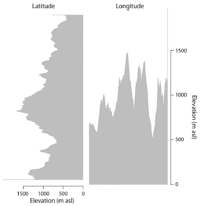
Figure 1
Mean elevation values of the study area according to the DEM used in this research for both rows (latitude) and columns (longitude)
3.2. The geographic distribution of weather stations
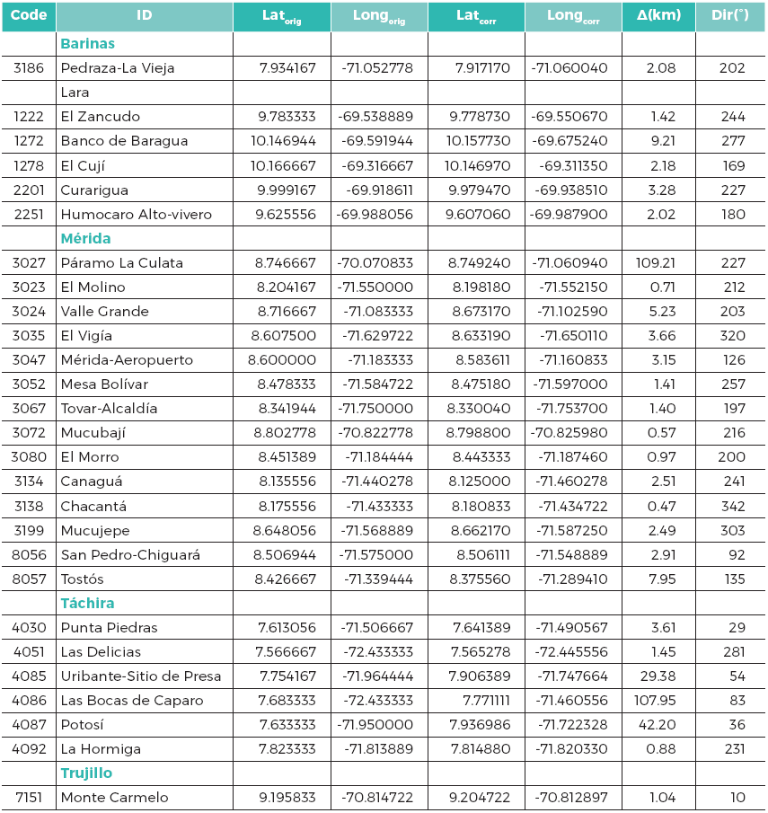
Of the 342 weather stations in the study area, 314 provided mean monthly precipitation data for at least one month for 10 or more years between 1950 and 2000, both years inclusive (Chart 1). The larger number of weather stations were located in Táchira (total 88/useable 81), followed by Mérida (76/71), Trujillo (67/61), Lara (62/60), Barinas (26/21), Portuguesa (19/17), Zulia (three/two), and finally Apure (one/one). We detected that at least 27 (8.6 %) of these 314 weather stations required some correction with regards of the geographic coordinates provided by their metadata. The mean distance of these 27 corrections was of 12.9 km, within a range from 0.5 km (Station serial 3138 «Chacantá») to 109.2 km (Station serial 3027, «Páramo La Culata», whose original geographic coordinates provided in the metadata located it in the Barinas’ Llanos).
Nearestneighbor distancesamong weather stations range from 0.28 km to 30.14 km, median 4.18 km and third quartile8.39 km. The comparison between the empiric distribution of the nearest neighbor distances, Ĝobs(r), and the theoretical cumulative distribution function, Ḡ(r), indicated that a portionof the weather stations were distributed randomly, while the remnant ones were slightly clustered so long as part of the empiric distribution lied above the mean, including the critic rank, suggesting an excess of short distances among nearest neighbors (Figure 2). This observation was reinforced by the aggregation index of the nearest neighbor (Clark & Evans, 1954), whose calculated value was 0.88. It is noteworthy that when this index lies above one indicates uniformity; one indicates randomness and below one indicates clustering of the point pattern.
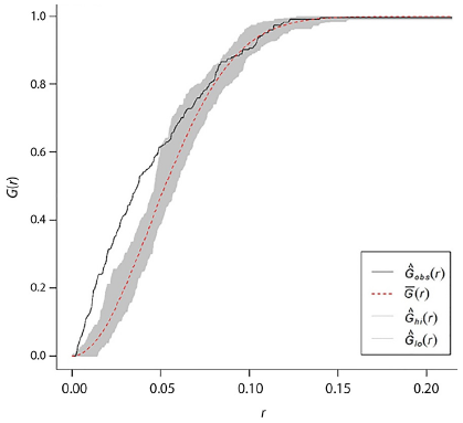
Figure 2
Comparison between the observed distances among nearest neighbors, Ĝobs(r), and the theoretical cumulative distribution function, Ḡ(r), with a confidence rank established sing Monte Carlo simulations (Ĝlo(r) – Ĝhi(r))
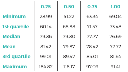
The spatial density distribution of weather stations measured through kernel smoothing (Bivand et al., 2008) demonstrated the dependency of local estimates of density on band amplitudes: narrow amplitudes yielded more extreme values, while wide amplitudes reduced the interquartile ranges (Chart 2). Furthermore, this dependency also was observed in figure 2, where low sigma values highlighted a greater density (clustering) of weather stations in Táchira State as well as along the longitudinal valleys.
When comparing graphically the distribution function of the elevation values of our DEM against the distribution function of the weather stations elevations (Figure 3), our results suggested that the study area was adequately represented throughout the elevation range, except for the most extreme heights. Such observation was corroborated by the two-sample Kolmogorov-Smirnov test (D = 0.28; p = 0.281).
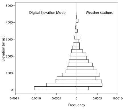
Figure 3
Comparison of the elevation distributions of both the pixels in DEM (right) and the location of weather stations (left) in the study area
3.3. Mean monthly precipitation values
Mean monthly precipitation throughout the year showed a drier period among December-March, being wettest the rest of the year (Figure 4). The greatest variability observed in the June-August quarter reflected the diffe rences between the unimodal precipitation regime of Llanos slope and the bimodal pattern of the Maracaibo’s Lake slope with its characteristic short dry season around August. On the other hand, Figure 4 also suggested the absence of aberrant mean monthly precipitation values, which could represent erroneous measures, suggestion shared by the histograms in Figure 5 which additionally highlighted that mean monthly precipitation is positively skewed for all months.
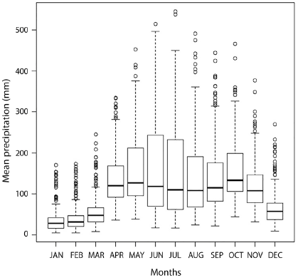
Figure 4
Variation of the mean monthly precipitation in the study area throughout the year
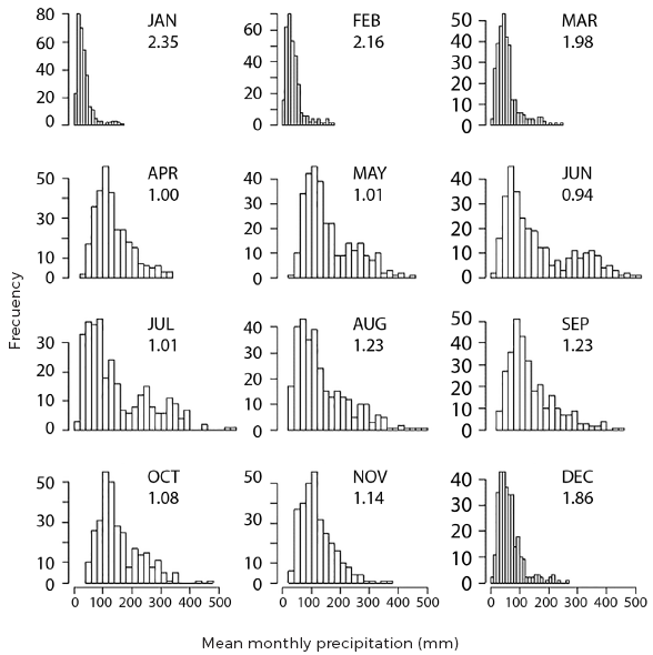
Figure 5
Histograms and skewness corresponding to the mean precipitation for each month
Furthermore, the presence of dubious values was also discarded by the bubble plots (Figure 6), which additionally demonstrated a displacement throughout the year of the mean monthly precipitation relative maxima: these are concentrated on the Maracaibo’s Lake slope at Táchira and Mérida in January, moving gradually toward the Llanos slope during the subsequent months, where they are concentrated by June to August, returning gradually back to Maracaibo’s Lake slope by December.
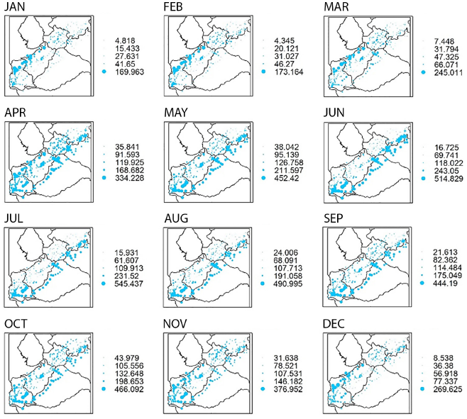
Figure 6
Bubble plots of the mean precipitation for each weather station for each month
3.4. Precipitation and geographic distribution
According to Moran’s I coefficients (Gittleman & Kot, 1990), the mean monthly precipitation values were spatially autocorrelated in the study area (p< 0.0001 for all cases; Chart 3), averaging 0.183 within a range between 0.147 (March) and 0.206 (June). On the other hand, mean monthly precipitation and elevation were correlated for any month (Figure 7).
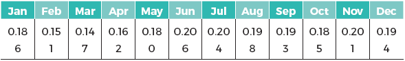
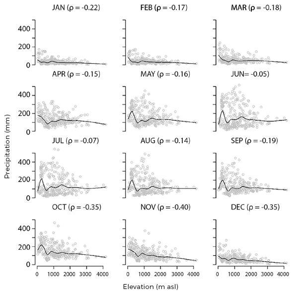
Figure 7
Spearman correlation between mean monthly precipitation and elevation, contrast highlighted through a loess curve
4. Discussion
Although a greater number of weather stations would always be desirable, our analysis indicated that the amount and geographic distribution of the weather stations providing relevant information can be considered adequate, for example, to be used to generate reliable mean monthly precipitation interpolations. This is a surprising finding given that the climatological network was not set ad hoc to accomplish such target.
Effectively, Burrough & McDonnell (1998) suggested that at least 50 to 100 samples are required to yield a stable variogram, while Webster & Oliver (1992) indicated that 100 samples are the minimal amount needed as to generate reliable estimations, although in the case of a normally distributed isotropic variable 150 samples are enough and 225 samples are reliable. Therefore, the amount of samples, that is, the 314 weather stations with relevant information on mean monthly precipitation available in the study area exceeds by far the minimal requirements to generate reliable interpolations.
On the other hand, although Englund et al. (1992) indicated that the spatial distribution pattern of samples (random, stratified or regular) has a worthless effect on the performance of some spatial interpolation techniques such as the ordinary kriging, others have indicated the opposite (Li & Heap, 2014), because variograms are sensible to sample clustering degree when, for example, there is heteroscedasticity or a relationship among the local mean and the data variance (Goovaerts, 1997). Thus, an intensive sampling or great proportion of clustered samples are convenient in the case of data with variogram with short range, while variograms with wide range require few samples distributed more uniformly (Marchant & Lark, 2006).
Moreover, Li & Heap (2011) indicated that an irregular sampling pattern, or samples spatially distributed accordingly to the degree of variability of the primary variable in a given region, would be preferable than a uniform sampling pattern. Otherwise, samples could be excessively dispersed as to identify the correlation and result in a pure nugget (Webster & Oliver, 2007), reducing the precision of the predictions (Gotway et al., 1996), because a wider space among samples implies less information in the resulting maps (Li & Heap, 2014). Thus, a spatial sampling pattern excessively dispersed can yield interpolated surfaces much more variable in those areas with high density of samples than in areas where such density is low, resulting in structures which are nothing but artifacts due to the configuration of data (Li & Heap, 2014).
In such a sense, the weather stations evaluated in the present study were located following an adequate pattern which was almost random, with a slight tendency to clustering specially in the Táchira State as well as along the longitudinal valleys where the dynamics of winds and other phenomena may result in deep differences within short distances with regards of precipitation characteristics.
The distribution of the weather stations along the elevation gradient also indicated an adequate sampling pattern. In fact, only lowest and highest heights were underrepresented, but the first constituted the surrounding lowlands with more homogeneous precipitation characteristics, while the last occupied a very small portion of the study area.
Mountains influence regional climates modifying the precipitation patterns: intercepted wind trades are forced to ascend, cool down, saturate (given that cold air holds a lower humidity tan warm one) and precipitating most of their humidity on windward slopes, to descend thereafter throughout the leeward slopes as a cold and dry air mass that picks up the humidity in the environment (Vivas 1992). This situation explains why there was correlation between elevation and mean monthly precipitation for any month in the study area.
The World Meteorological Organization (2012) standards indicate that for regional models, observational data must have a resolution of at least 10 km, and must be representative of significant portions of the region of interest. Considering the nearly random distribution of the weather stations throughout the study area, with three quarters of them being separated 8.39 km or less from its nearest neighbors, and distributed along most the elevation gradient, the data on precipitation available in the study area fulfilled such standards.
Finally, Guerra et al. (2009) defined the climatic information available for Venezuela as ‘scarce and little reliable’ both at temporal and spatial scales, especially in the case of the Andean region, as a result of an insufficient climatologic network, short recording series and problems with the information gathering. Our results contradicted, at least partially, such asseverations for the period 1950-2000, although available data suggests that most of the weather stations under INAMEH responsibility stopped to generate information thereafter.
Acknowledgements
We are deeply indebted to Professors Herbert Hoeger, Mayerlin Uzcátegui, Giorgio Tonella, Kay Tucci and Francisco Hidrobo for providing computing facilities. Doctors Luis Fernando Chaves Sanabria, María Angelina Pacheco and Julia Chacón Labella provided us with fundamental literature. This article is dedicated to the memory of Professor-Herbert Hoeger (1959-2015). This research was fundedby the Consejo de Desarrollo Científico, Humanístico, Tecnológico y de las Artes, CDCHTA of Universidad de Los Andes, Project codeC-1911-14-01-B.
6. References quoted
BERMÚDEZ, M. A.; VAN DER BEEK, P. & M. BERNET. 2011. «Asynchronous Miocene-Pliocene exhumation of the central Venezuelan Andes». Geology, 39(2): 139-142.
BIVAND, R. S.; PEBESMA, E. J. & V. GÓMEZ-RUBIO. 2008. Applied Spatial Data Analysis with R. Springer, New York. USA.
BRUMMITT, N. & E. N. LUGHADHA. 2003. «Biodiversity: Where’s hot and where’s not». Conservation Biology, 17(5): 1.442-1.448.
BURROUGH, P. A. & R. A. MCDONNELL. 1998. Principles of geographical information systems. Oxford University Press, Oxford.
CINCOTTA, R. P.; WISNEWSKI, J. & R. ENGELMAN. 2000. «Human population in the biodiversity hotspots». Nature, 404(6781): 990-992.
CLARK, P. J. & F. C. EVANS. 1954. «Distance to nearest neighbour as a measure of spatial relationships in populations». Ecology, 35(4): 445-453.
DIGGLE, P. J. 2003. Statistical analysis of spatial point patterns. Arnold. London, UK.
DIXON, P. M. 2002. «Nearest neighbour methods». In: A. H. EL-SHAARAWI & W. W. PIEGORSCH (eds.). Encyclopedia of environmetrics. pp. 1.370- 1.383 John Wiley & Sons. New York, USA.
ELITH, J. & J. R. LEATHWICK. 2009. «Species distribution models: ecological explanation and prediction across space and time». Annual Review of Ecology, Evolution and Systematics, 40: 677-697.
ELITH, J.; PHILLIPS, S. J.; HASTIE, T.; DUDÍK, M.; CHEE, Y. E. & C. J. YATES. 2011. «A statistical explanation of MaxEnt for ecologists». Diversity and Distributions, 17(1): 43-57.
ENGLUND, E.: WEBER, D. & N. LEVIANT. 1992. «The effects of sampling design parameters on block selection». Mathematical Geology, 24(3): 329-343.
FRANKLIN, J. 2009. Mapping species distributions: spatial inference and prediction. Cambridge University Press. Cambridge.
GITTLEMAN, J. L. & M. KOT. 1990. «Adaptation: statistics and a null model for estimating phylogenetic effects». Systematic Zoology, 39(3): 227-241.
GOOGLE INC. 2014. Google Earth (version 7.1.2.2041). Available at: http://www.google.com/earth/download/ge/agree.html 20 July 2013.
GOOVAERTS, P. 1997. Geostatistics for natural resources evaluation. Oxford University Press. New York, USA.
GOTWAY, C. A.; FERGUSON, R. B.; HERGERT, G. W. & T. A. PETERSON. 1996. «Comparison of kriging and inverse-distance methods for mapping soil parameters». Soil Science Society of America Journal, 60(4): 1.237-1.247.
GUERRA, F.; GÓMEZ, H.; GONZÁLEZ, J. & Z. ZAMBRANO. 2009. «Modelización de la distribución de la precipitación para el estado Táchira utilizando SIG’s y geoestadística». Geoenseñanza, 14(2): 293-318.
GPSYV. 2013. VENRUT. Mapas de Venezuela para GPS ruteables (version 13.07). Available at: http://www.gpsyv.net25 July 2013.
HASTENRATH, S. 1984. «Interannual variability and annual cycle: mechanisms of circulation and climate in the tropical Atlantic sector». Monthly Weather Review, 112(6): 1.097-1.106.
HIJMANS, R. J.; CAMERON, S. E.; PARRA, P. J.; JONES, P. G. & A. JARVIS. 2005. «Very high resolution interpolated climate surfaces for global land areas». International Journal of Climatology, 15: 1.965-1.978.
HUBER, O. & M. A. OLIVEIRA MIRANDA. 2010. «Ambientes terrestres de Venezuela». In: J. P. RODRÍGUEZ, F. ROJAS SUÁREZ & D. G. HERNÁNDEZ (eds.). Libro rojo de los ecosistemas terrestres de Venezuela. Provita, Compañías Shell in Venezuela and Lenovo Venezuela, Caracas, Venezuela.
INSTITUTO NACIONAL DE METEOROLOGÍA E HIDROLOGÍA (INAMEH). Climatología, datos de precipitación mensual. Caracas, Venezuela..
JARVIS, A.; REUTER, H. I.; NELSON, A. & E. GUEVARA. 2008. Hole-filled SRTM for the globe (version 4). Available from the CGIAR-CSI SRTM 90m Database: http://srtm.csi.cgiar.org. 15 July 2013.
JIMÉNEZ, N. & J. E. OLIVER. 2005. «South America, Climate of». In: J. E. OLIVER (ed.). Encyclopedia of World Climatology. Encyclopedia of Earth Sciences series. pp. 673-678. Springer. Dordrecht.
JOHANSSON, B. & D. CHEN. 2003. «The influence of wind and topogr aphy on precipitation distribution in Sweden: statistical analysis and modeling». International Journal of Climatology, 23(12): 1.523-1.535.
LI, J. & A. D. HEAP. 2011. «A review of comparative studies of spatial interpolation methods in environmental sciences: performance and impact factors». Ecological Informatics, 6(3-4): 228-241.
LI, J. & A. D. HEAP. 2014. «Spatial interpolation methods applied in the environmental sciences: A review». Environmental Modelling & Software, 53 (March): 173-189.
MARCHANT, B. P. & R. M. LARK. 2006. «Adaptive sampling and reconnaissance surveys for geostatistical mapping of the soil». European Journal of Soil Science, 57(6): 831-845.
MEEK D. W. & J. L. HATFIELD. 1994. «Data quality checking for single station meteorological database». Agricultural and Forest Meteorology, 69(1-2): 85-109.
MONASTERIO, M. & S. REYES. 1980. «Diversidad ambiental y variación de la vegetación en los páramos de los Andes Venezolanos». In: M. MONASTERIO (ed.). Estudios Ecológicos en los páramos andinos. pp. 47-91. Editorial de la Universidad de Los Andes. Mérida, Venezuela.
MYERS, N.; MITTERMEIER, R. A.; MITTERMEIER, C. G.; DA FONSECA, G. A. B. & J. KENT. 2000. «Biodiversity hotspots for conservation priorities». Nature, 403: 853-858.
OLSON, D. M. & E. DINERSTEIN. 1998. «The global 200: a representation approach to conserving the Earth’s most biologically valuable ecoregions». Conservation Biology, 12(3): 502-515.
PETERSON T. C.; EASTERLING, D. R.; KARL, T. R.; GROISMAN, P.; NICHOLLS, N.; PLUMMER, N.; TOROK, S.; AUER, I.; BOEHM, R.; GULLETT, D.; VINCENT, L.; HEINO, R.; TUUOMENVIRTA, H.; MESTRE, O.; ALEXANDERSSON, H.; JONES, P. & D. PARKER. 1998. «Homogeneity adjustments of in situ atmospheric climate data: A review». International Journal of Climatology, 18(13): 1.493-1.517.
PRUDHOMME, C. & D. W. REED. 1999. «Mapping extreme rainfall in a mountainous region using geostatistical techniques: a case study in Scotland». International Journal of Climatology, 19(12): 1.337-1.356.
PULIDO, N. 2014. «Bordes urbanos metropolitanos en Venezuela ante nuevas leyes y proyectos inmobiliarios». Cuadernos de Geografia, 23(1): 15-38.
QUANTUM GIS DEVELOPMENT TEAM. 2013. Quantum GIS Geographic Information System. Open Source Geospatial Foundation Project. Available at: http://qgis.osgeo.org 15 July 2013.
R DEVELOPMENT CORE TEAM. 2014. R: A language and environment for statistical computing. R Foundation for Statistical Computing. Vienna. Available at: http://www.R-project.org 12 May 2014
REDAUD, L.; DE ROBERT, P.; MOTHES, M.; MAYTIN, C.; MATOS, F.; MONTILLA, M.; MONASTERIO, M. & I. GARAY. 1991. «Caracterización del sistema de producción agrícola de Los Nevados, Sierra Nevada de Mérida, Venezuela». In: J. SAN JOSÉ & J. CELECIA (eds.). Enfoques de ecología humana aplicados a los sistemas agrícolas tradicionales del trópico americano. pp. 153-198. CIET. Caracas, Venezuela.
RODRÍGUEZ, N. & G. DEFIVES. 1996. «Zonas y patrones climáticos en la región andina». Economía, 11: 139-152.
SILVA LEÓN, G. A. 2010. Tipos y subtipos climáticos de Venezuela. Escuela de Geografía, Universidad de Los Andes. Mérida-Venezuela. Trabajo de ascenso a la categoría de Titular. (Inédito).
ŠTĚPÁNEK, P.; ZAHRADNÍČEK, P. & P. SKALÁK. 2009. «Data quality control and homogenization of air temperature and precipitation series in the area of the Czech Republic in the period 1961-2007». Advances in Sciences and Research, 3(1): 23-26.
TAYLOR, M. A. & E. J. ALFARO. 2005. «Central America and the Caribbean, Climate of». In: J. E. OLIVER (ed.). Encyclopedia of World Climatology. Encyclopedia of Earth Sciences Series. pp. 183-188. Springer. Dordrecht.
VIVAS, L. 1992. Los Andes venezolanos. Academia Nacional de la Historia. Caracas, Venezuela.
WEBSTER, R. & M.A. OLIVER. 1992. «Sample adequately to estimate variograms of soil properties». Journal of Soil Science, 43(1): 177-192.
WEBSTER, R. & M. A. OLIVER. 2007. Geostatistics for environmental Scientists. John Wiley & Sons, Ltd. Chichester.
WORLD METEOROLOGICAL ORGANIZATION. 2012. «Technical regulations. Basic documents». N° 2. Volume .1 General meteorological standards and recommended practices. WMO No. 49. Geneva, Switzerland.
ZAR, J. H. 1999. Biostatistical analysis. Prentice Hall. New Jersey, USA.