Introduction

The present research work arises from an interest in the history and role of fiscal policy, particularly the tax system. Taxation is a way of providing the necessary resources to support the functions of a state, but it should also be conceived as a tool to promote economic development. Therefore, it is necessary to examine the issue of taxation and economic growth in the Colombian case.

In the literature, important authors stand out for their contribution to the topic of economic growth and taxes, such as Barro (1990), Saquib et al. (2014), and Koester and Kormemdi (1989), among others. Their approaches converge in analyzing the interaction between public spending, taxation, and growth, highlighting the existence of a non-linear relationship in which taxes can affect economic growth both positively and negatively. While an efficient tax structure can finance productive investments and strengthen state capacity, an excessive or poorly designed tax burden can generate distortions, discourage private investment, and reduce capital accumulation, thus limiting economic dynamism.

In recent years, the incidence of taxes on economic activity has been a central topic of discussion. However, empirical evidence is still scarce. Employing an endogenous economic growth model that includes taxes on consumption and corporate profits, we intend to contribute to the topic.

Based on the above, this research aims to analyze the incidence of direct income tax and indirect value-added tax on Colombia's economic growth between 1970 and 2023. To this end, a vector error correction (VEC) model is used, which suggests that indirect taxes have a negative effect on economic growth while direct taxes have a positive effect.

The paper is divided into seven sections, including this introduction. This is followed by a review of theoretical literature on the subject and the model of economic growth with taxes. The third section presents different national and international empirical studies. The fourth section presents a descriptive analysis of the evolution and trend of the gross domestic product and the collection of each tax. The fifth section indicates the methodology used and the results of the econometric estimations for Colombia. Finally, sections five and six present the study's conclusions and recommendations.

Theoretical framework

The interest in analyzing the impact of taxes on economic growth was first presented by the economic scholars who have developed the well-known new growth theory, among them Barro (1990), who laid the foundations of an endogenous growth model that considers public sector spending and the role of taxes on it. In this sense, he begins his approach by arguing that public services play a fundamental role in the formation of private-sector production. It is through this role that Barro (1990) observes how potentially beneficial state intervention in the provision of these services can be for economic growth.

For this reason, he proposes a model of economic growth in which he considers that total production is given by a combination of private capital and the number of public services provided by the State, with constant returns to scale but diminishing returns to each factor. However, the existence of the assumption of constant returns becomes more consistent if it is assumed that private capital is composed of human capital and physical capital.

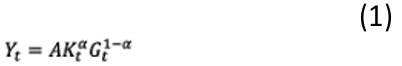
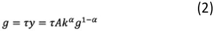
Equation 1 represents the total production function, which follows the structure of the so-called classical function where K^□ is the private capital which, as mentioned above, is composed of physical and human capital and G^□-□ which refers to the number of public services provided by the central government. Thus, it is assumed that the state has a balanced budget, this means that it finances its public spending with direct or indirect taxes over time. This is expressed in per capita terms in Equation 2.

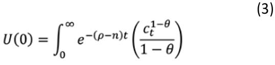
Also, this model considers that the representative household has an infinite fida within the context of a closed economy in which households seek to maximize utility. In this way, the model alludes to the fact that economic agents consider public spending an exogenous variable since it is not determined by them but by the State. This is expressed in Equation 3.

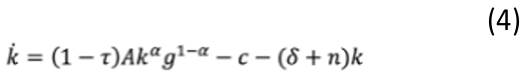
Then, if the household budget constraint is considered, it will reflect the maximum production achieved minus the total production paid to the State in the form of taxes, so the remainder must be distributed between consumption and investment as follows in Equation 4:

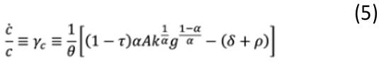
Hence, the growth rate of consumption is always constant at any point in time because □ is constant, and □ grows at a constant rate, so g must grow equivalently. The intuitive reason is that the tax converts an increase in income into an increase in government revenue, and this, in turn, becomes spending as seen in Equation 5.

Barro and Sala-i-Martin (2004) present an endogenous growth model that includes government functions and taxes. The government is assumed to have a balanced budget in which it finances expenditures with taxes. They consider proportional taxes on vwage income ( τ_w ), income from private assets ( τ_a ), consumption (τ_c ), y las and corporate profits ( τ_f); they assume that tax rates are constant over time.

The presence of taxes and transfers modifies the budget constraint of the representative household, which maximizes a substitution utility function. With the first-order condition of the Hamiltonian, the consumption growth rate is obtained as in Equation 6.

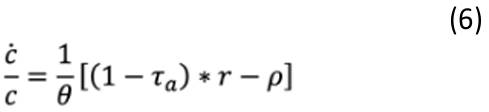
Therefore, the household's decision depends on the after-tax rate of return (1 - a)*r and a discount factor p. However, the consumption tax rate does not affect the individual's choice over time since it is constant. Otherwise, if the tax rate is expected to increase in the future, they will want to consume more today and less tomorrow so that consumption growth will be reduced.

Romer (1986; 1990) presents a long-run growth model in which knowledge is assumed to be an input to production with increasing marginal productivity. It is essentially a competitive equilibrium model, but with endogenous technological change, and unlike the other models, growth rates can increase over time. There are three types of agents in this class of economies: producers of final goods who use technology with labor and a set of intermediate goods that they must rent, inventors of capital goods who own a patent once created (monopoly power), and consumers who choose the quantity they wish to consume and save to maximize the utility function. This approach is used in the economic growth model, which will be constructed later with income tax and value-added tax as a feature of the production function.

Economic growth model with direct income tax and indirect tax on value added

Next, an endogenous economic growth model incorporating taxes is constructed. The model is characterized by the integration of neoclassical families and firms in imperfect (monopolistic) competition, based on the research of Barro, Sala-i-Martin, and Romer exposed above. The taxes considered here are proportional levies on consumption (Τ_f), and firms' profits (Τ_c); indirect the former and direct the latter.

Households

In this model, Equation 7 shows that the inhabitants of the economy maximize a utility function of the form:

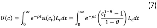
The utility of individuals is the sum of their instantaneous utility functions, discounted at the rate p the infinite time horizon. The population growth rate is constant and equal to n , so that , at time t , is given by . And □ is a const ant describing the desire to smooth consumption over time.

The total income of a household can be used for consumption or for the acquisition of financial assets (a) that generate an interest rate r. Thus, the per capita budget constraint of individuals in the presence of taxes is given by Equation 8:

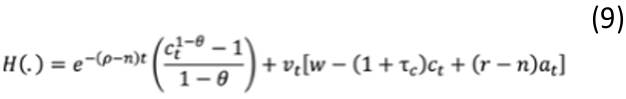
The problem of simple dynamic optimization can be solved with the Hamiltonian method; it is a reformulation of Lagrangian mechanics, where the control variable is consumption (c), and the state variable is the stock of assets (a). Equation 9 illustrates this:

The first-order conditions in this case are as follows in Equations 10 through 14:

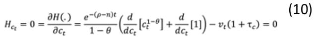
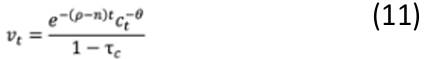
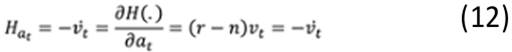
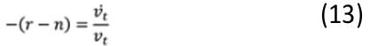
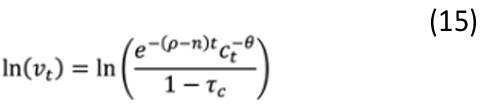
Equation (14) expresses the transversality condition, which means that optimizing individuals does not want to leave anything of value after their death because they could have consumed it to increase their utility. Also, we operate with logarithms on both sides of Equation (11). The results are Equations 15 and 16:

Where the gross consumption tax growth rate , in Colombia has been gradually changing over time due to the various tax reforms implemented. We now derive with respect to time and arrive at the following equation: 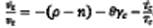. This expression is substituted into (11) to arrive at the consumption growth condition in Equation 17:

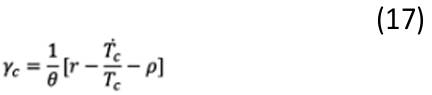
Therefore, the household's decision depends on the rate of return, the Value Added Tax rate, and the discount factor (p).

Firm Sector

Firms in the economy behave like Romer's model (seen previously), where technology is interpreted as a formula or knowledge. The inventors of capital goods invest certain resources in research and development (R&D) and then own a patent that gives them market power. Therefore, the final product is under perfect competition, while the production of inputs is monopolistic competition. There are two types of markets.

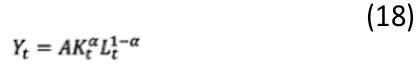
The first one is the final production market. It considers that producers of final goods face a production function that is in the classical Cobb-Douglas type production function. Where A is a parameter measuring the efficiency of the firm, L_t is labor, and K_t is a composite of aggregate intermediate goods. This is represented in Equation 18.

The composition of aggregate intermediate goods considered in is given by Equation 19:

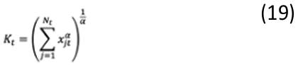
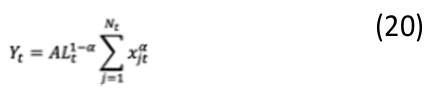
Where N is the number of goods invented so far; hence, there is no destruction of ideas. And X is the quantity of the intermediate good that firms demand and buy. If we substitute K in the final production function of Equation 18, we obtain Equation 20:

Firms hire labor in a competitive market and buy each intermediate good p_jt. Combining these factors of production, they obtain the product sold at a price (p_y,t = ); they are price-accepting. Therefore, the profits obtained are represented in Equation 21:

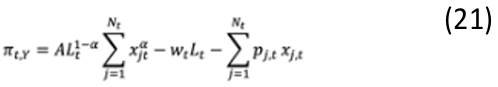
In this equation Wt Lt are the labor costs and are the costs for using intermediate goods. To obtain the optimal demands of L_t and X_j,t , Equation (21) is derived with respect to each.

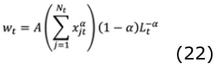
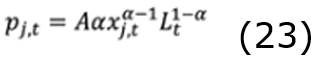
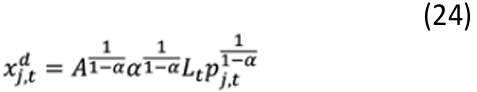
Equation 22 is the demand for labor, it is assumed to be inelastic; for any given wage level, wt. Equation (23) can be rewritten to express the demand for intermediate goods as a function of their own price and the parameters A, L y □ . The result is Equation 24.

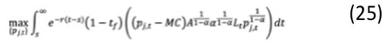
The second market is the input production market. It considers the firms that produce the intermediate goods. Once the product is invented, they can sell it at a desired price to infinity, considering the cost per unit; MC (marginal cost). The only restriction is that the price cannot be too high because the demanders (the producers of the final good) will not buy too many units. In this market profits are equal to the quantity produced multiplied by the selling price (p_j,t) minus the quantity produced multiplied by the marginal cost of each unit. Considering the firm's profit tax, the inventors' maximization program for deciding the price of a product is pictured in Equation 25:

To simplify the notation MC=1. Since there are no dynamic constraints in this problem, the first- order conditions require that the derivative of the term inside the integral with respect to the price be zero:

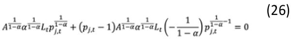
From Equation 26 several terms can be simplified. Rewriting this optimality condition, we obtain the profit-maximizing monopoly price in Equation 27.

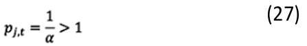
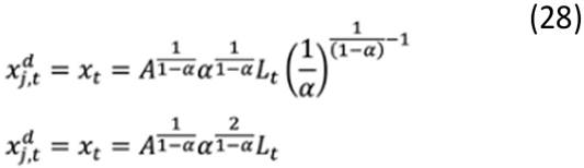
All invented products have the same price and will be higher than the marginal cost (given that □ □□), so inventors can recover l+D costs. Substituting the price (27) in the demand function (24), the effective quantity sold of each intermediate product is obtained in Equation 28:

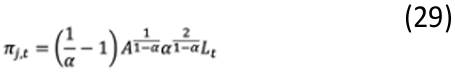
The quantity produced by each of the intermediate producers is the same. Substituting this in Equation (25), we obtain that the instantaneous profit is identical for all and constant over time. This is representeded in Equation 29

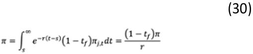
Therefore, the present value of these benefits reflects that after inventing a new product, the inventor knows Equation 30:

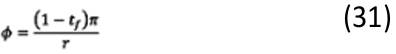
If there is perfect competition in the business of being an inventor, the condition of free entry into the market will equal the expected net income with taxes , with the cost of l+D; denoted by the letter. Therefore Equation 31:

Finally, if r is replaced by according to (29) in (19), we find the consumption growth rate in Equation 32:

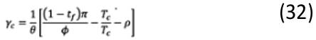
Hence, the consumption growth rate is a function of the corporate income tax (T_f), the consumption tax (T_c), and the constant parameters affecting the saving rate through impatience and the desire to smooth consumption, p and □. In equation 31, the negative relationship between tax rates and the consumption growth rate is evident.

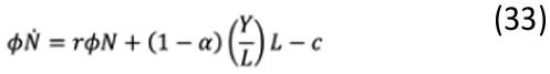
Finally, in general equilibrium, the growth rates of GDP and technology must be equal to the growth rate of consumption. The equilibrium condition in the financial market requires that the total assets held by consumers (b), are equal to the only asset that has a positive net supply which are the inventing firms . At the same time, the wage is given by 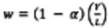. 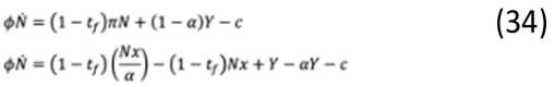The above is substituted into the consumer constraint 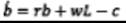to obtain the aggregate of the economy in Equation 33.

The value of r is obtained from Equation 31, and at the same time, □ is substituted according to Equation 29 considering that the second term from the right is x. This is illustrated in Equation 34:

Consequently it is taken into account that, the quantity produced of each of the intermediate producers is 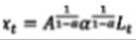and the production is 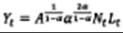. In this way we obtation Equation 35:

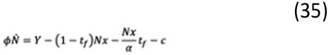
The total production is distributed in consumption, in the production of a quantity x of each of the intermediate products invented with the presence of tax and in the resources used in the research process . Dividing the two sides of Equation 35 by N , we obtain that in the steady state, all the terms of the equation are constant because the growth rate of N is constant. Hence, . Since output is proportional to N, the growth rate of output is also equal to the growth rate of consumption .

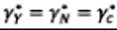Therefore, Equation 36 confirms the negative relationship between tax rates and the economy's growth rate.

Empirical literature

Helms (1985) analyzes the effect of state and local taxes on economic growth. He uses a growth model that considers the government budget constraint to rank the offsetting effects of taxes and spending applied at the state level. It relies on a pooled time series and cross-sectional data for 48 U.S. states between 1965 and 1979, incorporating variables such as income, government spending, transfers, fiscal variables, wage rates, unionization, and population density. As a result, it indicates that the effects of taxes on a state's economy depend to a large extent on the proportionate use of revenues. Thus, increases in state and local taxes reduce economic growth when revenues are used to finance transfer payments. However, when revenues are used to fund public services (such as education, health, and roads), they can counteract the disincentive effects of taxes. This indicates that taxes cannot be studied in isolation and underscores the importance of considering the incentives provided by a state's expenditures.

García-Escribano and Mehrez (2004) analyze the impact of the size of the public sector and the composition of spending and revenue on economic growth. They followed the standard literature approach using five-year averages for estimation and thus avoided correlations created by the business cycle. They use panel data for 18 OECD countries between 1970 and 2002 that include factors such as the annual growth rate of GDP per capita, non-fiscal variables such as labor force growth, and the ratios of spending, surplus, and income to GDP. The results indicate that the tax burden should be supported mainly by indirect rather than direct taxes because the latter are more distorting. Business (direct) taxes negatively affect investment, in contrast to a subsidy that would lead to economic incentives and, thus, a growth of the labor force. Thus, taxes affect economic growth through investment and employment.

Saquib et al. (2014) researches the effects of taxes on economic activity in Pakistan. They employ three models to estimate the effects of tax structure on different economic activities. The first is the growth model, which incorporates investment, tax-to-GDP ratio, public services, inflation, and labor force. The second is the investment model, which includes income tax, GDP, interest rates, and inflation. Finally, the consumption model integrates disposable income and sales taxes. For this, they used time series data from 1973 to 2010. They concluded that taxes negatively affect consumption, investment, and GDP because an increase in sales tax leads to an increase in prices and thus a decrease in consumption. On the income tax side, it generates disincentives to invest, given the lower disposable income.

Bleaney et al. (2001) examine the impact of fiscal policy on growth as a function of the structure of taxes and expenditures. They evaluate endogenous growth models that classify budget elements as distortionary or non-distortionary taxes and productive or non-productive expenditures. Distortionary taxes affect agents' investment decisions concerning physical and/or human capital, thus distorting the steady-state growth rate. Contrary to non-distortionary taxes, which do not affect saving/investment decisions due to the nature of the preference function. To estimate the impact, they used a panel data set for 22 OECD countries between 1970-1995, considering the implications of government budget constraints to avoid biases in the regression coefficients. As a result, the effect of fiscal policy on growth depends on how it is financed, i.e., if it is financed by a combination of non-distortionary taxes and non-productive expenditures, an increase in productive expenditures significantly improves growth, and an increase in distortionary taxes significantly reduces growth.

Koester and Kormendi (1989) analyze the effects of average and marginal tax rates on the growth rate of economic activity (the "shape" of the growth path) and the level of economic activity (the "location" of the growth path). They use what is known as supply-side economics, which distinguishes two tax rates: the average tax rate, which is the ratio of tax revenues to GDP, and the marginal tax rate, which is an estimate of a linear time-series regression of tax revenues on GDP. To do this, they used a set of 33 countries between 1970 and 1979. They show that a decrease in tax progressivity causes an increase in economic growth, and an increase in marginal tax rates negatively impacts the level of economic activity, i.e., holding average tax rates constant, higher (lower) marginal tax rates are generally associated with parallel downward (upward) changes along the growth path.

For Colombia, we add Fergusson's (2003) and Granger et al. (2018) works. The former evaluates the impact on economic growth and welfare of tax policy in Colombia. It uses a macroeconomic representative agent methodology to calculate average effective tax rates if the economy has three goods: consumption, labor, and capital. It uses annual data on tax revenues and tax bases between 1970 and 1999. Then, it uses these rates to evaluate the welfare and economic growth costs of taxation based on a simple dynamic general equilibrium model with the assumption of perfect foresight. The results show an increasing behavior of average effective tax rates over the period, especially in the 1990s, and a decline in economic growth due to tax policy.

Granger et al. (2018) determine the fiscal policy stance (countercyclical or procyclical) in Colombia. They use cointegration techniques based on adjustments to the statutory rates of the main national taxes, which directly reflect the decisions of the tax authority. For the empirical evaluation, they use variables such as statutory rates of national taxes, government spending, gross debt, Gross Domestic Product, capital stock, economically active population, and the Gini coefficient between 1970 and 2017. From the tax information, they constructed three indexes that capture the behavior of rates according to the share of each tax in total revenue and the statutory rate adjustments they made in the different reforms. The results indicated that fiscal policy was procyclical in Colombia for the study period because most of the reforms approved coincided with periods of economic slowdown. Thus, tax policy has responded not only to product cycles but also to other factors, such as the size of the fiscal deficit or the need to cover the increase in public spending.

Delestre et al. (2022) studied the behavior of direct and indirect taxes in the United Kingdom since 2023. Using descriptive statistics and the calculation of the Gini coefficient, they find that some taxes are progressive². Among the results, they highlight that the direct income tax is progressive and does not generate distortions in the market since they mention that the average tax rates increase as a function of income, which makes the tax reduce inequality in the income distribution.

Methodological framework

This research develops the methodological framework through a descriptive and econometric analysis of the relevant economic variables for Colombia from 1970 to 2023. To study the impact that taxes have had on economic growth. We consider the taxes that contribute most to total tax collection, such as income tax and value-added tax, and to quantify their effect on economic growth, we use the gross domestic product.

The choice of the Colombian economy as the object of study is justified by the growing trend of direct and indirect taxes during the fifty-three years covered by this research. During this period, it is possible to identify patterns consistent with the theoretical framework previously presented, wherein higher growth in the tax collection rate and lower economic growth rates are observed.

The sources of economic information used in this research come from the Banco de la República de Colombia (BanRep) and the Dirección de Impuestos y Aduanas Nacionales (Dian). The series included the collection of direct income tax, indirect value-added tax, and GDP adjusted to 2015 prices. The series are expressed in millions of current pesos in Colombian currency, so it was necessary to deflate the variables to avoid strengthening the figures due to inflationary pressures. The latest consumer price index of 2015 was used for the tax series. With respect to GDP, retropolation techniques were used to chain the series, considering the methodologies of 1975,1995, 2005, and 2015 as the base year for the calculation of GDP.

Description of data

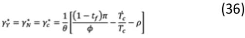
Figures 1 and 2 show that the gross domestic product has fallen significantly during 1975, 1991, 1999, and 2020. In these periods, on the one hand, it can be observed that the increase in direct and indirect taxes has been greater. On the other hand, the variation of the highest peaks in GDP growth occurred in the seventies of the twentieth century and the first decade of the twenty-first century. In 1992-1999, the coffee sector entered an irreversible decline, which caused the economy to show a significant decrease in 1999, while oil exports grew gradually. Therefore, in the first decade of the XXI century, the supply of exportable goods gradually shifted from coffee to the mining-energy sector. The new sector has led to a sustained increase in real income since the foreign investment attracted by this sector has a multiplier effect on the rest of the economy. However, because of the pandemic, the confinements, and the restrictions on the country's economic activity, the GDP again registered a significant decrease by 2020.

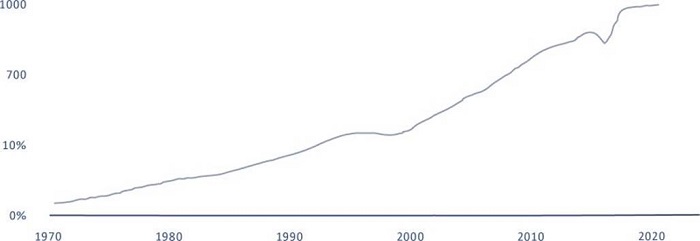
Figure 1.
Gross domestic product trend during 1970and 2023
Note. Figure expressed in millions of Colombian pesos. Source: Own elaboration based on Ban Rep data. (2024).

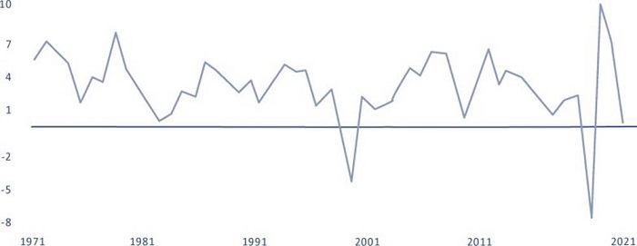
Figure 2.
Year-on-year gross domestic product growth rate during 1970 and 2023
Note. Figure expressed in percentages. Source: Own elaboration based on Ban Rep data (2024).

The tax system in Colombia is divided into national and municipal taxes. The former are issued by the executive branch and subject to consideration by the national congress for approval. There are two types of national taxes: direct and indirect. Direct taxes are levied on the income and wealth of individuals and/or legal entities. They are called direct because they are applied directly to individuals. Indirect taxes are levied on production, services rendered, imports, and consumption. These taxes in Colombia are not based on the taxpayer's ability to pay. Therefore, income tax is a direct tax, and value-added tax is indirect.

According to Figures 3 and 4, it can be interpreted that the income tax has had a sustained increase over time; however, the highest increases are observed in 1975,1991, and 2023, where this tax grew 64.5%, 71.4%, and 42.6%, respectively. The common factor of these increases is attributed to the tax reforms that have increased this tax from Alfonso López Michelsen's government to Gustavo Petro Urrego's current administration.

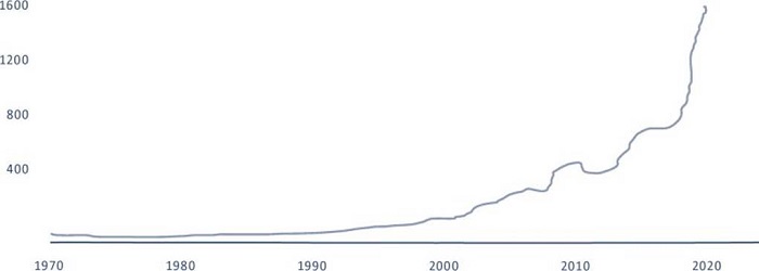
Figure 3.
Direct income tax trend during 1970 and 2023
Note. Figure expressed in millions of Colombian pesos. Source: Own elaboration based on Ban Rep data (2024).

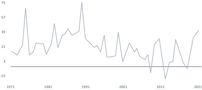
Figure 4.
Year-on-year growth rate of direct income tax during 1970 and 2023
Note. Figure expressed in percentages. Source: Own elaboration based on Ban Rep data (2024).

In the same line, Figures 5 and 6 show that the value-added tax has maintained a constant growth since this tax refers to the price that the producer has put on what he offers; this price must cover the production costs and generate a profit that allows him to sustain his business. In this sense, it had its highest growth rates in 1975,1996, and 2022, where this tax grew 102.5%, 53.8%, and 22.3%, respectively.

Collection has shown a considerable growth trend since the end of the 1970s due to the gradual increase in the general rate. Because the government intended to tax more internal goods to replace the tax on external goods as a result of the process of economic liberalization. The highest peak in revenue growth occurred in the seventies of the twentieth century with 67.9%, when the base of taxed products was expanded, and the general rate increased from 3% to 15%. The value-added tax, as well as the income tax, has undergone several modifications in the period analyzed, such as in 1983, the general rate was lowered to 10%, but services and retail trade were included in the list of taxed products, while in 1990 the rate increased to 12%. Subsequently, in 1992, the general VAT rate went from 12% to 14%; it continued increasing to 16% in 1995, and in 2016 a significant change was made, increasing the tax rate from 16% to 19%, generating a lower taxation of the tax.

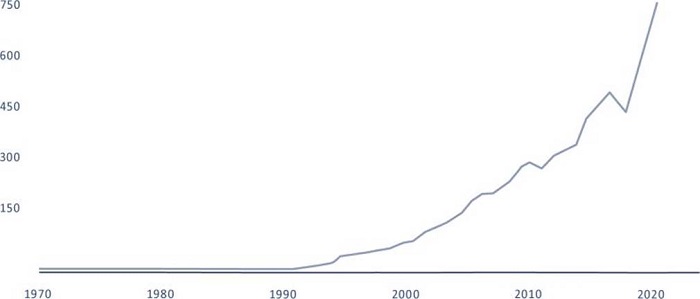
Figure 5.
Indirect value-added tax trend during 1970and
Note. Figure expressed in millions of Colombian pesos. Source: Own elaboration based on Ban Rep data (2024).

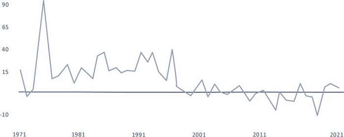
Figure 6.
Year-on-year growth rate of indirect value-added tax during 1970and 2023
Note. Figure expressed in percentages. Source: Own elaboration based on Ban Rep data (2024).

Finally, an exhaustive description of the impact and summary of the study variables can be seen in Table 1. In the first place, it is expected that, because of an increase in the collection of value-added tax, the gross domestic product will be reduced since, according to García-Escribano and Mehrez (2004), this tax may generate distortions in the market, indirectly affecting the final consumer and his or her ability to pay or disposable income.

Table 1.
Summary and expected impact of variables

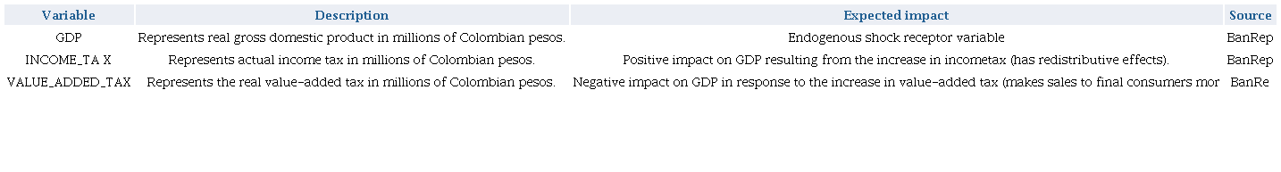
Source: Own elaboration.

Variable	Description	Expected impact	Source
GDP	Represents real gross domestic product in millions of Colombian pesos.	Endogenous shock receptor variable	BanRep
INCOME_TA X	Represents actual income tax in millions of Colombian pesos.	Positive impact on GDP resulting from the increase in incometax (has redistributive effects).	BanRep
VALUE_ADDED_TAX	Represents the real value-added tax in millions of Colombian pesos.	Negative impact on GDP in response to the increase in value-added tax (makes sales to final consumers mor	BanRe

Secondly, it is expected that an increase in direct income tax collection will increase economic growth since, according to Delestre et al. (2022), this tax can generate greater tax equity, given that it is a progressive tax, which does not generate distortions in the market since it is levied on people with a greater capacity to pay, and therefore does not modify their consumption decisions.

Econometric model

To empirically evaluate the impact of direct income tax and indirect value-added tax on economic growth, we follow the study proposed by Saquib et al. (2014), who studied the effects of taxes on economic activity in Pakistan, and Granger et al. (2018) who identified the position of tax policy in Colombia. Based on these investigations, an extension is carried out using a multivariate time series model type VEC, with the objective of quantifying the impact generated by an increase in the tax collection of these taxes on economic growth in Colombia from 1970 to 2023.

Model estimation

Within the multivariate time series models, we find the VEC reference models, which are widely used when studying time series that are integrated, that is, variables that establish a long-term relationship with each other. This is the result of the simultaneity in which the multivariate calculation of the time series considers the dynamic effect of a shock or unanticipated innovation on one of the variables that integrate the system on the other.

For this reason, the empirical structure of the model used in this research is configured, where a vector of endogenous variables is considered to empirically evaluate the incidence of the increase in income and value-added tax collection on economic growth in Colombia. The VEC model used in this work is expressed in Equation 37:

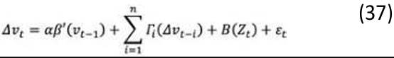
The subscript refers to the number of optimal lags for Colombia. On the left-hand side, it refers to the vector of endogenous variables of the system in differences at the time of the model, within which it refers to the direct income tax, the value-added tax and to the growth rate of real gross domestic product. On the right side, there is a vector that multiplies the transposed cointegration vector and the vector that represents the variables in levels in the period³. Also, there is a matrix that multiplies the vector of variables in the first difference, and finally, the coefficient matrix, involves dichotomous variables that can model seasonal effects to control the effects of extreme outliers⁴.

However, it must be understood that the coefficients associated with the VEC models can report a series of large values that call for a joint analysis of these through the quantification of the short- and long-term impact of the random shocks on the explanatory endogenous variables, as well as understanding how these stochastic perturbations affect the evolution of the system's variables. For this last aspect, it is necessary to estimate the long-run equilibrium function, the adjustment speed equation, the impulse-response functions, and finally, proceed with the Cholesky variance decomposition method.

Tests performed

When estimating multivariate time series models, verifying a series of assumptions through statistical tests is essential to ensure their robustness. First, the order of integration of the variables must be determined, which is crucial to specify whether the variables should be estimated at levels with intercept or trend in first or second differences. In this research, since a VEC model is estimated, the variables should have unit roots in their levels; however, they should not have unit roots in the first differences. To corroborate this, we use the Phillips-Perron test⁵ with the transformed variables. We apply a natural logarithm to each one to confirm that they are not stationary in levels but are stationary when the first difference is considered.

Once it is confirmed that the series have unit roots in levels and are stationary with the first difference, it is necessary to determine the optimal number of lags for the VEC model. This is accomplished using the Chi-square test for lag exclusion⁶, where p-values of less than 5% are used. While the p-values suggest using between one and four lags, according to Helms (1985), following the estimation of his growth model with annual data, he employs five lags for estimation.

Next, the order of cointegration of the system variables must be verified. For this, the Johansen test (1995⁷) was used, specifically the trace test and the maximum eigenvalue to define the number of potential cointegration relationships in the model. In the case of this research, it was verified thatthere is at least one long-term cointegration relationship, with which we proceeded to estimate the VEC model⁸.

Subsequently, the dynamic stability of the model is verified, ensuring that the variables return to their dynamic equilibrium levels in the long run after identifying variations in the vector of innovations. In our research, we estimate the inverse roots of the autoregressive polynomial⁹ to confirm the stability of the VEC model.

Next, two additional assumptions of the VEC model are reviewed. First, we evaluate whether the variance of the residuals is constant using White's heteroscedasticity test¹⁰ without cross terms, concluding that the residuals are homoscedastic. Second, the absence of serial correlation is verified using the Lagrange Multiplier test¹¹, confirming that there is no autocorrelation between the lags applied in the model.

Finally, the normality test¹² was performed on the model residuals, which evaluates the asymptotic distribution of the residuals in the estimated VEC model. This step is based on complying with the assumptions of uncorrelated errors and homoscedasticity, as suggested by Johansen (1995), who points out the importance of verifying that the residuals do not deviate significantly from the white noise assumption. To meet this assumption, this research performed a detailed review of the outliers in the residuals of the VEC model to create the dichotomous exogenous normality variables included in the model. Likewise, the test is performed to confirm this assumption's fulfillment and validate the residuals' normality.

Analysis of results

Once the corresponding tests have been carried out to verify the proposed model's consistency, we analyze the impact of the increase in income and value-added tax collection on economic growth. In this sense, argumentation based on the empirical and graphical evidence resulting from the impulse- response functions is presented, considering the impact of this shock twenty years ahead.

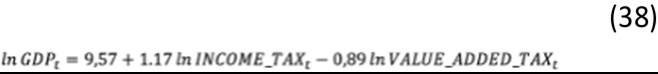
First, once it is determined that the three variables of this research present an order of integration and identify that there is a cointegration relationship and, therefore, a cointegration vector, which indicates the long-run equilibrium (1 -1.17 0.89), which means that the long-run equilibrium function of the incidence of the increase in income tax and value-added tax collection on economic growth in Colombia is pictured in the Equation 38:

Now, the macroeconometric model estimated in this research has the same specification of the Johansen cointegration test, the VEC model is as follows in Equation 39:

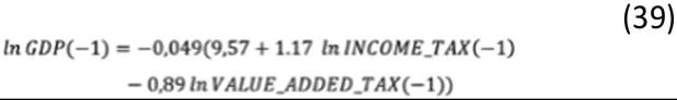
Where 0.049 is the speed of adjustment and is statistically significant. The closer to zero, the faster the equilibrium is reached in the long run. In turn, as mentioned above, the residuals of the estimated VEC model, as a result, have zero order of integration in the long run, indicating that the cointegration relationship has no unit root, which means that these series are cointegrated in the long run and, therefore, Equation (35) is a correct specification of the function of the impact of the increase in income and value-added tax on economic growth for Colombia.

In this sense, if direct income tax collection is increased by 1%, gross domestic product growth would increase by 1.2%, thus showing a direct relationship between direct taxes and economic growth. On the other hand, if the value-added tax is increased by 1%, the gross domestic product contracts by 0.9%, showing an inverse relationship between indirect taxes and economic growth.

This is consistent with the literature since direct taxes provide a stronger automatic stability than indirect taxes because they have a higher elasticity to the economic cycle. For example, income tax during a recession reduces people's disposable income so that they will pay less in taxes. In addition, this analysis is supported by impulse-response functions, which consider the incidence of these taxes on Colombia's economic growth with a projection horizon of twenty periods ahead (20 years later).

Accordingly, Figure 7 allows us to interpret that the gross domestic product positively reacts more strongly to an income tax shock. This effect is noticeable from the first year; however, it took its highest initial value from the second year, going from 0.006 percentage points (p.p.) at that time to 0.019 p.p. in the seventh year. It is observed that the reaction remains positive between 0.010 and 0.014 p.p. during the twenty periods of the projection horizon.

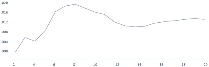
Figure 7
Impulse-response function of an income tax shock on economic growth
Source. Own elaboration.

On the other hand, Figure 8 shows that the gross domestic product reacts less strongly to a negative value-added tax shock. In this sense, it can be interpreted that the impact of an increase in this tax reduces the gross domestic product by 0.0129 p.p. in the seventh year, after which it can be observed that the negative impact is maintained throughout the estimated period.

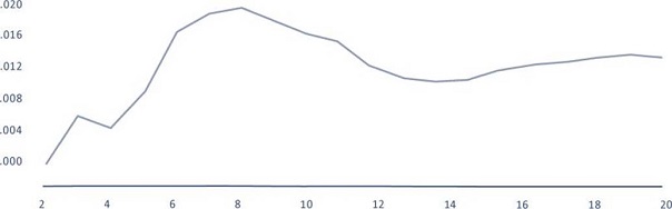
Figure 8.
The impulse-response function of a value-added tax shock on economic growth
Source. Own elaboration.

Finally, the previous results are compared with the Cholesky variance decomposition of the VEC model. This analysis strengthens the study's findings by examining how the endogenous variable vector evolves over a projected period of twenty years. The evidence suggests that, in year twenty, the variation in economic growth is explained by 14.34% due to changes in income tax collection, 0.92% due to changes in value-added tax collection, and 84.74% due to its own variations.

Conclusions

This study investigates the influence of income tax and value-added tax on economic growth in Colombia during the period from 1970 to 2023. It is based on modern growth theory, using an endogenous economic growth model that incorporates taxes on consumption and corporate profits. The Johansen (1995) cointegration methodology is used to carry out empirical investigations, focusing on the estimation of a VEC-type multivariate time series model.

The main results reveal that an increase in direct tax collection is positively related to higher economic growth. In contrast, an increase in indirect tax collection is associated with a decrease in economic expansion.

In addition, impulse-response functions and Cholesky variance decomposition show that, after 20 years of the increase, the impact on economic growth generated by an unanticipated increase in tax revenue is distributed as follows: direct income tax accounts for 14.34% of the variance, while indirect value-added tax accounts for 0.92%.

The findings suggest that the evolution of economic growth reacts similarly to increases in income tax and value-added tax; however, a greater positive intensity is observed in the impact of an increase in income tax on growth. Based on these results, it can be affirmed that in Colombia, there is a contraposition between the increase in indirect tax collection and economic growth but a positive correlation with respect to direct taxes.

Recommendations

Based on the research findings that suggest the need to restructure the tax system, it is recommended that a series of economic policies be implemented aimed at promoting a more equitable and favorable tax system for economic growth in Colombia. First, it is crucial to reduce dependence on value-added tax as the main source of revenue. To achieve this, one could consider implementing measures that gradually lower the general value-added tax rate and compensate for the loss of revenue through a greater focus on collecting direct taxes on income and business profits.

In addition, fiscal policies should be designed to counteract the regressivity of the value-added tax, ensuring that the tax burden is proportional to the income level of taxpayers. This could be achieved by implementing graduated tariff schemes or introducing tax exemptions for lower-income sectors. The possibility of establishing tax refund mechanisms for low-income taxpayers could also be explored as a way to mitigate its regressive impact.

On the other hand, a greater diversification of tax revenue sources should be encouraged, seeking to reduce excessive dependence on indirect taxes. This could involve exploring new ways of taxing wealth, such as implementing property or financial transaction taxes, which could contribute to a more equitable distribution of the tax burden and greater stability in government revenues. Ultimately, these policies should be part of a comprehensive approach that promotes inclusive and sustainable economic growth in Colombia.

References

Barro, R. J. (1990). Government spending in a simple model of endogenous growth. Journal of Political Economy, 98(5), 103-125. https://doi.org/10.1086/261726

Banco de la República. (2024). Producto Interno bruto 1970-2023. Banco de la República de Colombia. Recuperado de https://www.banrep.gov.co/es/estadisticas/catalogo#GDP2015

Bleaney, M., Gemmell, N., & Kneler, R. (2001). Testing the endogenous growth model:Public expenditu re, taxation, and growth over the long run. Canadian Journal of Economics/Revue canadienne d'économique, 34(1), 36-57. https://doi.org/10.1111/0008-4085.00061

Barro, R., & Sala-i-Martin, X. (2004). Economic growth second edition. http://ndl.ethernet.edu.et/bitstream/123456789/15298/1/29%20.%20Robert_J._Barro%2C.pdf

Delestre, I., Kopczuk, W., Miller, H., & Smith, K. (2022). Top income inequality and tax policy (No. w30018). National Bureau of Economic Research, https://doi.org/10.3386/w30018

Dirección de Impuestos y Aduanas Nacionales. (2024). Estadísticas de Recaudo Anual por Tipo de Impuesto 1970 - 2023. https://www.dian.gov.co/dian/cifras/Paginas/EstadisticasRecaudo.aspx

Fergusson, L. (2003). Impuestos, crecimiento económico y bienestar en Colombia (1970-1999). Desarrollo y Sociedad, (52), 143-202. https://www.redalyc.org/pdf/1691/169118076005.pdf

García-Escribano, M., & Mehrez, G. (2004). The impact of government size and the composition of revenue and expenditure on growth (IMF Working Paper No. 237(4), pp. 2-17). International Monetary Fund.

Granger, C., Hernández, Y., Ramos, J., Toro, J., & Zárate, H. (2018). La postura fiscal en Colombia a partir de los ajustes a las tarifas impositivas. Borradores de economía, 1038, 1-30. https://www.banrep.gov.co/sites/default/files/publicaciones/archivos/borradores_de_economia_1038.pdf

Helms, L. J. (1985). The Effect of State and Local Taxes on Economic Growth: A Time Series-Cross Section Approach. The review of Economics and Statistics, 574-582. https://doi.org/10.2307/1924801

Johansen, S. (1995). Identifying restrictions of linear equations with applications to simultaneous equations and cointegration. Journal of econometrics, 69(1), 111-132.

Koester, R. B., & Kormendi, R. C. (1989). Taxation, aggregate activity and economic growth: cross-country evidence on some supply-side hypotheses. Economic Inquiry, 27(3), 367-386. https://doi.org/10.1111/j.1465-7295.1992.tb01542.x

Romer, P. M. (1990). Endogenous technological change. Journal of political Economy, 98(5, Part 2), S71-S102. https://doi.org/10.1086/261725

Romer, P. M. (1986). Increasing returns and long-run growth. Journal of political economy 94(5), 1002-1037. https://doi.org/10.1086/261420

Saqib, S., AN, T, Riaz, M. F, Anwar, S., & Aslam, A. (2014). Taxation effects on economic activity in Pakistan. Journal of Finance and Economics, 2(6), 215-219.

Notes