Introducción

The business cycles are periodic (and irregular) fluctuations in the economic activity. They are characterized by the recurring rises and falls in the overall economy as well as the asymmetric behavior of these phases over time. Recessions tend to be deeper and more volatile, but less persistent and extensive than expansions, thus suggesting that phases are not necessarily identical (DeLong and Summers, 1986; Hamilton, 1989). While business cycles do not recur on a periodical basis and each cycle has unique characteristics, there are discernible regularities in their behavior through time. Business cycles last several years, and they often show repetitive patterns from cycle to cycle in the statistical movements of production, employment, profits and prices.

The analysis of business cycles is important for a number of different reasons. First, to determine cyclical fluctuations is essential for policy- makers in order to apply the proper macroeconomic policies. Second, to understand the behavior of the different Gross Domestic Product (GDP) components may help these policies to become effectively. For example, the pro-cyclical behavior of some these variables can help to propagate the benefits (or the damages) of macroeconomic policies implemented by governments. The opposite occurs if the behavior is anti-cyclical. Third, economies with similar business cycle characte-ristics may apply common macroeconomic policies, thus coordinating actions, efforts and initiatives to successfully cope adverse shocks.

Likewise, macroeconomic volatility is usually expensive in terms of well-being. This is particularly relevant for those economies with unequal income distribution or high poverty rates, which frequently lack of adequate instruments for stabilization policies (Toledo, 2008). In other words, the analysis of business cycles is not only important for the formulation of monetary and fiscal policies, but also for the design of social welfare systems as well as labor market policies.

Despite the existence of studies documenting the main stylized facts for a particular country in the past, the renewal interest in the analysis of the symmetries and asymmetries of business cycles emerged in the nineties when several regions of the world were involved in economic integration processes. The opinions have coincided that a certain degree of homogeneity and association between countries’ business cycles is essential for success of such processes. As a consequence, the existence of similarities in the business cycles has been considered a necessary condition for the harmonization of policies and institutions (see, for example, Mejía-Reyes, 1999; Arnaudo and Jacobo 1997).

However, the analysis of a common business cycle has not been a significant element in the economic research agenda in developing countries. As to Latin America, the studies on this topic have been relatively limited in past and they continue to be scarce in the present. In general, the existing studies suggest that there has not been a past common business cycle in Latin America. However, it is possible to find a common one for some subsets of countries, as suggested by several authors (see, among others, Engel and Issler, 1993; Arnaudo and Jacobo, 1997; Mejía-Reyes, 1999; Jacobo, 2002; Gomes Gutierrez, 2006; and Aiolfi et al., 2006).

Due to different reasons, notably the lack of interest in deepening the integration process in Latin America as a consequence of the dissimilar political perspective of party leaders, the analysis of common business cycles has disappeared from the regional literature.

In this paper, we perform a short —albeit important— statistical exercise and we try to document some properties about the regular cyclical movements of GDP in Argentina and Brazil for the period 1995-2018 on a quarterly basis. We study the co-movements between real GDP and its components for each of these two important econo- mies. The aim of our analysis is to determine whether the economic fluctuations follow a similar pattern according to their duration, intensity and timing.

We contribute to the literature in the following ways. First, we review the previous studies on the topic. Second, we report updated evidence on the main stylized facts about macroeconomic fluctuations in Argentina and Brazil, two of the most representative countries in the region, since the nineties. Recall that the nineties marked an era of globalization that clearly coincides with deliberative efforts to achieve a higher degree of trade and financial liberalization. As the world economy has become more and more integrated, the interdependence has increased and much of the world has moved in tandem. Hence, our interest is to study whether or not the co-movements between both economies exist. Third, while Hodrick and Prescott filter is applied to decompose the series into a trend and a cyclical component as usual, a minor novelty in our study is the use of a more reliable estimation procedure than the data-modification method in the X-11 to seasonally adjust the series called Seasonal and Trend (STL is its acronym) decomposition using LOESS.3

The rest of the paper is organized as follows. Section 1 briefly summarizes the literature on common co-movements on GDP in Latin America. Section 2 outlines the methodology. Section 3 presents the results. Section 4 concludes.

1. Literature review

In developing economies, the analysis of the business cycle has not been a standing element in the economic research agenda and the studies on this topic are relatively scarce in Latin America (Agénor, McDermott and Prasad, 2000; Catão, 2007).

On the one hand, some authors have focused on documenting the main stylized facts typically for a particular country. There are several works about this topic. Representative studies for Argentina include among others the work of Kydland and Zarazaga (1997), Cerro (1999), Capello and Grion (2003), Jorrat (2005), Diaz (2007), and Rojas, Zilio and Zubimendi (2009). As to Brazil, the most relevant examples are the papers of Val and Ferreira (2001), Ellery, Gomes and Sachsida (2002), Neumeyer and Perri (2005), and Souza-Sobrinho (2010). For brevity, we are not going to discuss each of these documents in this review.4 However, we will use them for comparative purposes regarding to our results, as we shall see in Section 4.

On the other hand, there are studies focusing on the presence of past asymmetries in the phases of Latin American business cycles. These include the works of Engel ad Issler (1993), Arnaudo and Jacobo (1997), Mejía-Reyes (1999), Agénor, McDermott and Prasad (2000), Cerro and Pineda (2002), Jacobo (2002), Gutierrez y Gómez (2009), Aiolfi et al. (2006), and González et al. (2012). Most of these studies not only analyze the correlations but also the underlying mechanism provoking business fluctuations through time.5

In an interesting paper, Engel and Issler (1993) analyze the short and the long-run co-movements of the GDP for Argentina, Brazil and Mexico. Among other findings, the authors suggest that these three countries share the same growth trend and business cycle.

However, according to Arnaudo and Jacobo (1997) this seems not to be the case for the Southern Common Market (MERCOSUR) coun- tries. They deal with the macroeconomic performance of these econo- mies (Argentina, Brazil, Paraguay and Uruguay, the four founding members) during twenty-five years. While there are a lot of discretion in obtaining the business fluctuations and the results may vary among different studies, when expansions and contractions are compared within countries their duration is variable and the degree of persistence is small. Besides, the relationship between GDP and each of its compo-nents (with the exception of consumption) seems to be poor. The simul-taneous relationships are different in time and size, although the authors find significant correlation of those for Argentina and Brazil.

As to Mejía-Reyes (1999), the author also finds a strong coincidence between the business cycles of Argentina and Brazil, and between the ones of Brazil and Peru, although he does not find any for the entire set. Precisely, he provides further evidence on the synchronization between business cycle regimes in seven American countries by using a classical business cycles approach. Despite the increase of interna- tional economic transactions within the continent, his results suggest that national business cycles are largely idiosyncratic (except for the United States and Canada). Thus, international macroeconomic policy coordination may not be effective, not at least in the short-run. Also, as a byproduct, he finds evidence of asymmetries between expansions and recessions in mean, volatility and duration of the business cycles in most of the countries.

With a different scope, Agénor, McDermott and Prasad (2000) document cross-correlations between macroeconomic fluctuations and other macroeconomic variables (such as fiscal variables, wages, inflation, money, credit, exchange rate and trade) for twelve develo- ping economies. They conclude that there are similar relationships with those observed in developed countries (counter-cyclical government expenditures, for example), as well as other results.6

In a motivating paper, Cerro and Pineda (2002) measure and explain to what extent Latin American countries’ growth cycles experienced co-movement in the last forty years, using different methodologies. They find that short-lasting cycles showed a great dispersion among cyclical correlation, while long-lasting ones displayed considerable co-movement. From the Structural Vector Autoregression approach, the results imply a very low degree of co-movement among the shocks affecting these economies. There exist important differences regarding to the speed of adjustment and to the volatility of demand shocks. According to the authors, Latin-American countries needs more policy coordination prior to any attempt to go further into an economic inte-gration process.

Jacobo (2002) deals with the macroeconomic behavior of Argentina, Bolivia, Brazil, Chile, Paraguay and Uruguay for twenty-seven years. According to the author, the arrhythmical beat among these economies in the past reveals there is little point in trying to align macroeconomic policies, thus concluding that the economies behave different.

More recently, Aiolfi et al. (2006) conducted a study for the most important Latin American economies in terms of GDP (Argentina, Brazil, Chile and Mexico). Throughout the results, they conclude that international economic interdependence and similar economic policies make the business cycles less volatile at the same time that these coun- tries have started a commercial and financial openness. These expec- table results tend to be in line with those suggested by Frenkel and Rose (1998).

It worth to mention the work of Gutierrez and Gómez (2009) who analyze the business cycles of the MERCOSUR’s members. Once the authors estimate the business cycles, they proceed to analyze them in order to see if there is some degree of synchronization. Despite the evidence of common features, the results suggest that the business cycles are not synchronized. This may generate an enormous difficulty to intensify the agreements in the MERCOSUR.

Likewise, González et al. (2012) analyze the synchronization of economic fluctuations in Latin America and present new evidence regarding the cyclical behavior of real GDP. Despite some important relations observed, the existence of a common cycle that invites us to think that full synchronization is not detected.

In a nutshell, the analysis of a common business cycle for Latin America is relatively scarce. The studies suggest the inexistence of a past common business cycle, notwithstanding the possibility to find a common one for some subset of countries as suggested by various authors.

2. Methodology

According to the standard analysis, it is possible to express the time series as the sum of four unobservable components:

(1)

where T_t is the trend, S_t is the seasonal component, C_t is the cyclical one and It is the irregular component (Enders, 1995). These four variables interact to produce the observe values of time series. Since we are interested in C_t, we need to eliminate the effect of other components.

Trend can be easily removed once the time series is seasonally adjusted (i.e. once we consider the pattern that exists when the series is influenced by seasonal factors) using standard techniques, as we are going to see. As to irregular variations, they usually follow a random pattern and, because of their unpredictability, attempt has not been made to study it mathematically. However, it should be noted that over a period of time, these random fluctuations tend to counteract each other and thus we may have a time series free of irregular variations.7

To define the business fluctuations, we need to extract its trend by some procedure. As proposed by Kydland and Prescott (1990), we use the Hodrick-Prescott (H-P) filter. This filter is one of the most popular statistical methods for time series to obtain the cycle.

In order to understand the framework of this technique, recall that it is necessary to consider the definition of the business cycle proposed by Lucas (1977). So, let y_t be a time series for t=1;2;...;T. If τ_t is the trend of this series, then the measure of business fluctuation is given by: c(t)=c_t=y_t-τ_t. Formally, the trend component of a series can be determined from the solution of the following minimization problem:

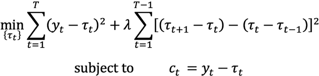(2)

being y_t the original series to be filtered, τ_t the trend component and ct the cyclical component of y_t.

The first component of the minimization problem is the cyclical component measured as deviations from the long-term path (which is expected to be, on average, close to zero in a long-run). The second part of the equation represents the variability of the trend penalized by the parameter λ. In the limit, when approaches infinity, the first differences (τ_(t+1)-τ_t ) tend to a constant and it is obtained as a solution to the problem. The choice of the value of λ depends on the frequency of the data. For quarterly data, Hodrick and Prescott propose to adopt the value of 1,600.

The H-P filter has a long history and different shortcomings have ben pointed out in the literature, as described by Ahumada and Garegnani (1999). We are not going into details regarding its drawbacks here. However, it may perhaps be noted without straying too far afield from our major focus that this technique can lead researchers to report apparent cyclical behaviors under certain circumstances (Harvey and Jaeger, 1993; Cogley and Nason, 1995).8 Moreover, Hamilton (2017) argues that one should never use the H-P filter as it results in spurious dynamics, has end-point problems and its typical implementation is at odds with its statistical foundations.

Notwithstanding the critics, Ravn and Uhlig (2001) suggest that none of the undesirable properties of the filter are particularly convincing and that the H-P filter has stood the test of time. Moreover, although elegant new bandpass filters have been developed (Baxter and King, 1999; Christiano and Fitzgerald, 1999), it is likely that the H-P filter remains one of the usual methods for detrending. Empirical practice with the H-P filter almost universally relies on standard settings for the tuning parameter that have been suggested largely by experimentation with macroeconomic data and exploratory reasoning. Its attributions clearly stem from three major facts. First, the filter can be used for estimating (and so removing) long term trends from macroeconomic time series. Second, a filter bandwidth can be specified (via a fixed value of the smoothing parameter) which is quite suitable in filtering terms for estimating trends with quarterly macroeconomic data. Third, it is important to highlight the fact that H-P filter allows us to easily compare the results with those of other works that have adopted the same methodology.

To use this procedure, the series must be previously seasonally adjusted. For this purpose, we employ the STL decomposition proce- dure to raw data prior to apply the H-P filter. Again, for the sake of brevity, some few words about this decomposition method follows.

A common technique to decompose a time series is the X-11 proce- dure, which was developed in the 1950s and 1960s and includes (at that time) modern statistical ideas, like the backing-fitting algorithm (itera- tive estimation of the trend, seasonal and regression components) or robust estimation. The STL method incorporates some new knowledge about backing-fitting which allows it to prevent the seasonal and trend components from competing for the same variation in the series.

The STL method incorporates iterated weighted least-squares, which is according to Cleveland et al. (1990) “a more reliable estima- tion procedure than the data-modification method used in X-11 (The X-11 robust estimate of location uses the sample standard deviation to determine the data modification, which is a poor method since the standard deviation can itself be very adversely affected by outliers)”.

We assume that the data, the trend component, the seasonal component and the remainder component are denoted by Y_t,T'_t,S_t and R_t respectively, and that, for t=1,…,n, the following relation holds:

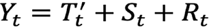(3)

STL basically consists of two recursive methods. In the first method a detrended series Y_t-T'_t is estimated. Then, the cycle-subseries of the detrended series is smoothed by LOESS regression.9 The collection of smoothed values for all the cycle-subseries is a temporary seasonal series named C_t. The next step involves three moving averages followed again by a LOESS smoothing applied to C_t, rendering the output series L_t. Afterwards the seasonal subseries is obtained by subtracting L_t from C_t (S_t=C_t-L_t) and finally the deseasonalized series Y_t-S_t is estimated.

The second iteration method provides robustness to the estimations. Having a first estimation of the remainder term R_t=Y_t-T'_t-S_t, a weight for each observed Y_t is defined in order to see how extreme R_t is. This robustness weight is defined as:

(4)

Then, the first recursive method is repeated, but in the smoothing procedures this weight ρt is employed to compute the LOESS regressions. The robustness iterations of the second method are carried out n₍₀₎ times.

As to the variable to be considered, we need to use one that is the most representative of the aggregate economic activity and the GDP in real terms seems to be the obvious candidate. Moreover, from the analysis of the correlation between GDP and its components we can obtained further information for our purposes. According to the litera- ture, we examine private and public consumption, investment, imports, exports, and trade balance.

With respect to statistical information, we use seasonally adjusted quarterly data from the first quarter of 1995 (1995.1) to the last quarter of 2018 (2018.4). The series have been obtained from the International Financial Statistics database of the International Monetary Fund.10 All the series are expressed in logarithms. Those variables that are not plausible to be transformed into their logarithmic form are expressed as a percentage of GDP.

As to the features of the business cycles, we consider the variability, persistence and the degree of association with the GDP fluctuation. We use the standard deviation to perceive the variability of each series, and the relative standard deviation to see if they are more (or less) volatile than output (i.e. if the relative standard deviation is greater than one, this would indicate that the variable is more volatile than GDP). The first order autocorrelation coefficient is used to measure the degree of persistence of the cyclical component of each variable.

We estimate the correlation coefficients ρ(j) for j=0; ±1; ±2; ±3;±4. Based on these estimates, the degree and direction of the movement of each variable is compared with GDP. When the contemporary values of the variable change in the same direction as those of the cycle’s indicator (ρ(j)>0), that variable is said to be pro-cyclical; when the change occurs in the opposite direction (ρ(j)<0), it is said to be counter- cyclical; and when the correlation coefficient is close to zero, it is said to be a-cyclical. We also determine if a variable precedes, follows or coincides with the actual GDP fluctuation. If ρ(j) reaches its maximum value for a j<0, the variable precedes the cycle. Similarly, if ρ(j) reaches its maximum value for a j>0, the variable changes after the cycle and follows the GDP cycle. Finally, if ρ(j) reaches its maximum value for j=0, the variable coincides with the GDP cycle.11

3. Results

In this section, we present the results for Argentina (subsection 3.1.) and Brazil (subsection 3.2.). Finally, we explore whether or not a certain degree of homogeneity and association exists between these economies (subsection 3.3.).

3.1. Argentina: Some stylized facts

First, we comment the country’s experience in terms of growth. Second, we present the correlations between GDP and its components to determine the strength of the relationships.

Figure 1 shows the evolution of Argentinean real GDP as well as its long-run trend. The real GDP has increased 100.77% and the annual average growth rate has been 2.78%.

GDP business fluctuations are presented in Figure 2. As seen, their intensity has varied throughout the period. During the first years, economic activity was below its long-term trend level due to the Tequila crisis in 1995. The activity experienced a recovery and reached a peak (of approximately 6%) in the second quarter of 1998 (1998.2). Argentina experienced a drop (15%) in 2001, when the convertibility plan was abandoned and the domestic currency depreciated. Due to the international crisis of 2008-2009, the economy was negatively affected and it suffered an additional drop (8%) in the second quarter of 2009 (2009.2). Thereinafter, the deviations of GDP with respect to its long-term trend level were not as deeply as before.

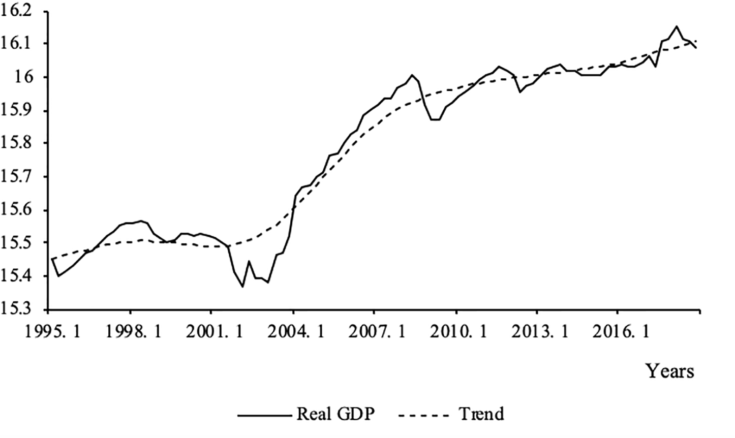
Figure 1
Argentina: Real Gross Domestic Product

(In logarithms of millions of 2010 pesos)

Source: Own estimates based on International Financial Statistics (IMF).

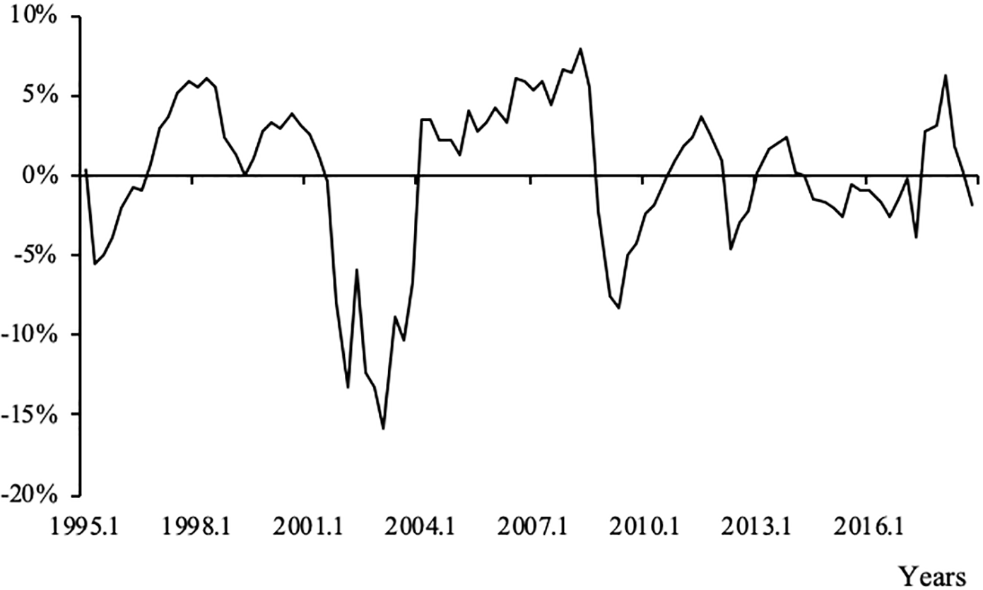
Figure 2
Argentina: GDP cyclical component
Source: Own estimates based on International Financial Statistics (IMF)

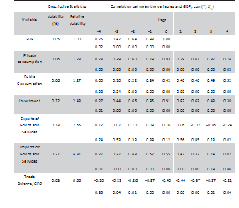
We complete the analysis with the study of the volatility of GDP and its components through their standard deviation. To this end, we summarize the results in Table 1. The table shows the volatility of each GDP component and trade balance as percentage deviation from its mean value (column 1), the relative volatility (column 2), the contemporaneous correlation coefficient between each aggregate demand component and GDP (column 3), and the phase shift of the series, which is obtained from the most significant estimated coefficients up to 4 lags and leads (column 4)12.

The table also shows that the volatility of GDP is 4.82%. It is higher than the volatility observed in earlier studies because our data includes crisis not previously considered by other authors. Imports present the highest volatility (20.7%).

However, it is important to observe the relative volatility of the variables (private and public consumption, investment, exports, imports and trade balance) as well as to estimate the correlation coefficients to establish the pro-cyclical, counter-cyclical or a-cyclical nature of GDP components as well as their movement with respect to GDP.

Table 1

Argentina: Cyclical behavior of real GDP and its main components(1995.1-2018.4

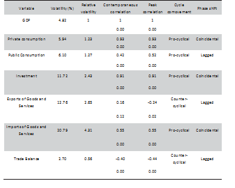
Source: Own estimates based on International Financial Statistics (IMF)

Private consumption is 23% more volatile than GDP and presents a high contemporaneous correlation with GDP (0.93). Thus, private consumption has a strong positive correlation with GDP and it is coincidentally and pro-cyclically¹³. This is a common characteristic in Latin American countries. Our results are similar to those of Aguiar and Gopinath (2007), and to the findings of Kydland and Zarazaga (1997). Figure 3 helps us to graphically perceive the association between private consumption and GDP.

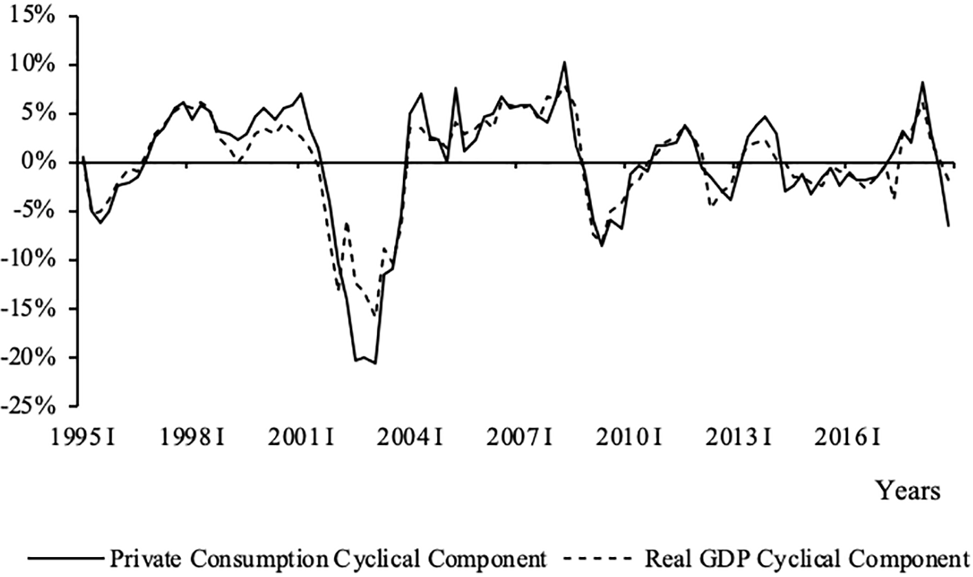
Figure 3
Argentina: GDP and Private Consumption cyclical components
Source: Own estimates based on International Financial Statistics (IMF)

Public consumption is 27% more volatile than GDP and presents a contemporaneous correlation (0.42). The literature finds a positive correlation as we do (Kydland and Zarazaga, 1997). Moreover, it exhibits a lagged correlation, which could indicate that public consumption follows the cycle of GDP (fourth quarter), as suggested by Rojas, Zilio and Zubimendi (2009). This pattern clearly results in the pro-cyclicality of fiscal policies and it tends to exacerbate the underlying economic cycle (Frankel, Vegh and Vuletin, 2011). Figure 4 lets us appreciate the pro-cyclicality behavior of public consumption.

As to investment, the volatility is almost 2.4 times greater than that of GDP, with a positive contemporary correlation (0.91). This result implies that the investment presents a contemporary and pro-cyclical behavior, coinciding with the results obtained by Fanelli and Frenkel (1996), Kydland and Zarazaga (1997), Loayza, Fajnzylber and Calderón (2004) and Rojas, Zilio and Zubimendi (2009). Such behavior can also be perceived in Figure 5.

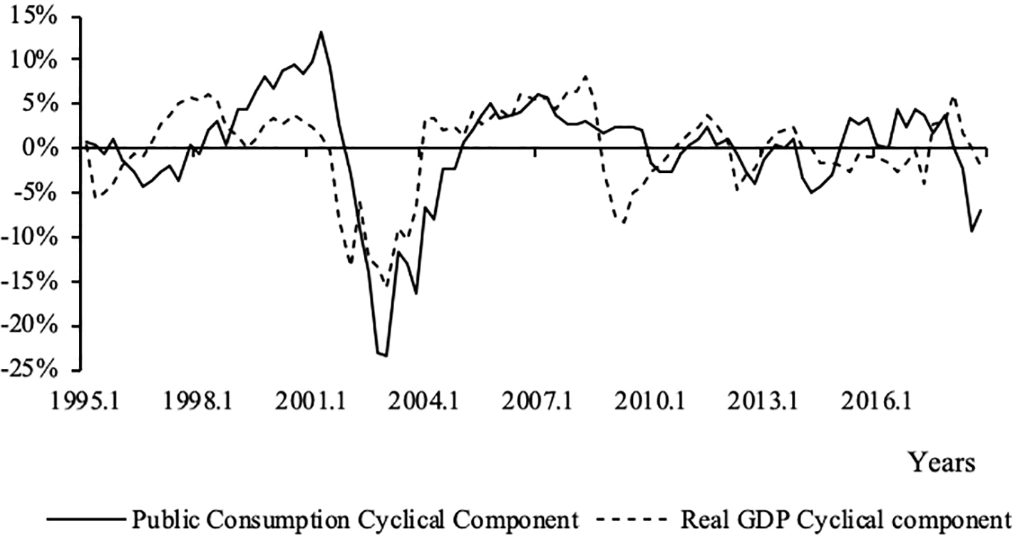
Figure 4
Argentina: GDP and Public Consumption cyclical components
Source: Own estimates based on International Financial Statistics (IMF)

As to the external variables, imports are nearly four times more volatile than the product (4.31) and exports are more than twice and a half (2.65)¹⁴. Imports are positively and contemporaneously correlated (0.55) with GDP. However, exports do not exhibit any significant correlation coefficient and they seem to follow an a-cyclical pattern and probably they are lagged with respect to GDP (fourth quarter). Anyway, we have to be cautious when interpreting these results because a myriad of different situations may have influenced throughout the period. In fact, Diaz (2007) suggests that exports become strongly pro-cyclically in a context where a devaluation exists. Such context is present in our sample in the periods 2002-2007 and in 2018.

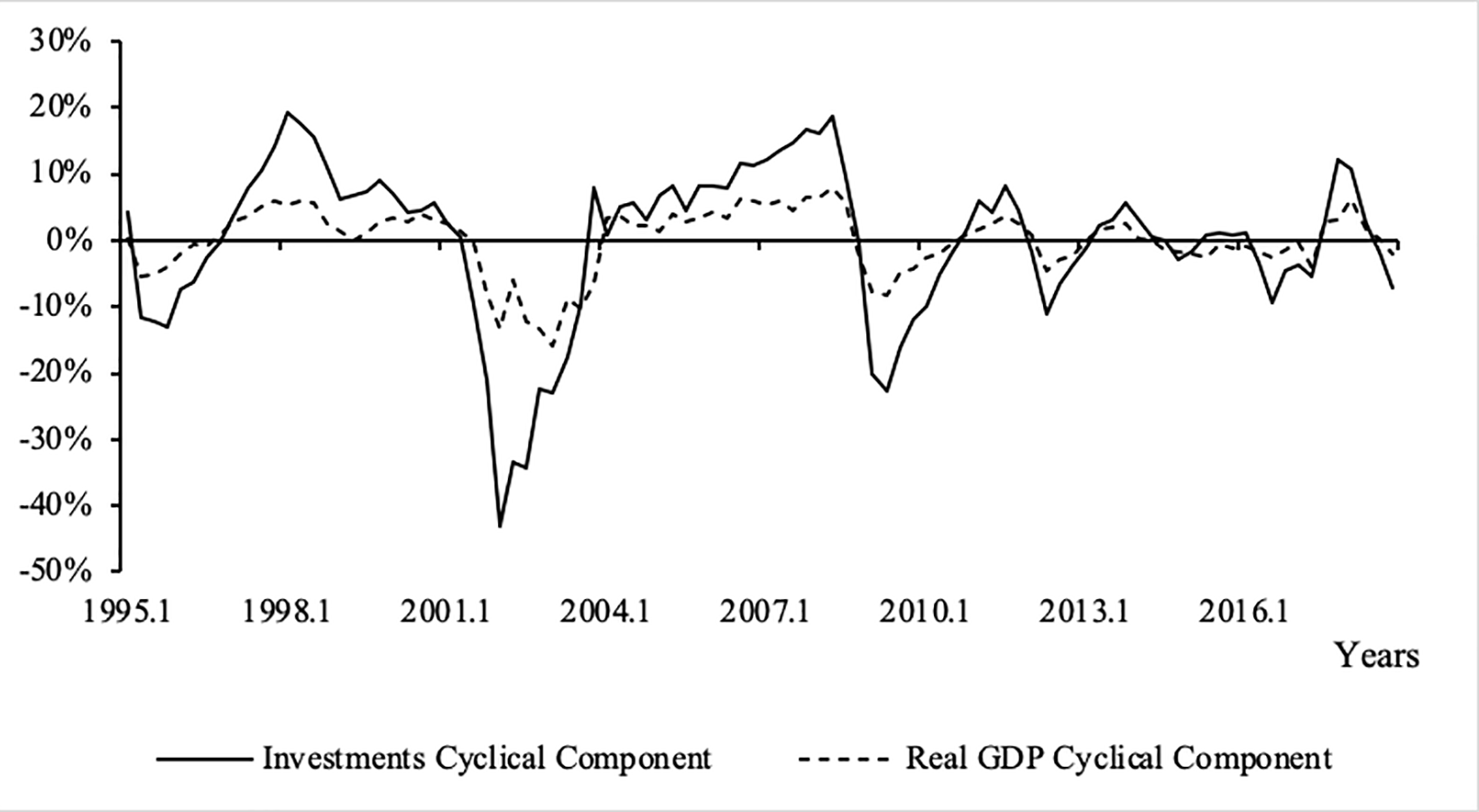
Figure 5
Argentina: GDP and Investment cyclical components
Source: Own estimates based on International Financial Statistics (IMF)

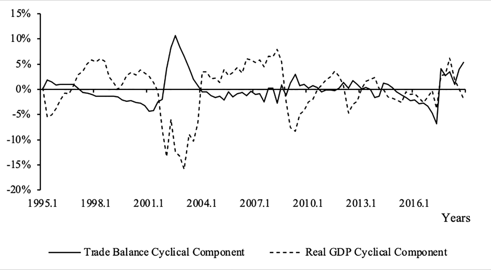
Figure 6
Argentina: GDP and Trade Balance cyclical components
Source: Own estimates based on International Financial Statistics (IMF)

Trade balance is less volatile than GDP (0.56) and have a counter- cyclical and a lagged (one quarter) behavior, as observed in Figure 6. It must be noted that the characterization of net exports as an anti-cyclical variable responds to the common properties in the business cycles of the region, and it is a result found by most of the studies.

To this respect, Arbatli (2009) argues that these findings are probably the result of negative shocks on GDP that, under credit restrictions, lead to a counter-cyclical trade balance response. Toledo (2008) explains that the sources of these shocks, particularly for Latin American economies, are the fluctuations in the terms of trade because the region is very vulnerable to their movements.

3.2. Brazil: Some stylized facts

As in the previous subsection, we firstly comment the country’s experience in terms of growth. Then, we present the correlations between GDP and its components to determine the strength of their relationships.

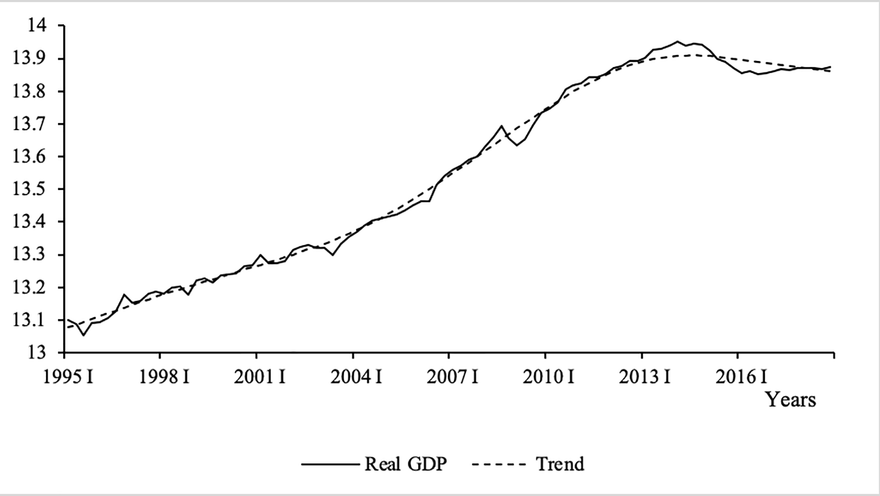
Figure 7
Brazil: Real Gross Domestic Product

(In logarithms of millions of 2010 reales)

Source: Own estimates based on International Financial Statistics (IMF)

As depicted in Figure 7, Brazil’s real GDP has increased 78.86%, with an annual average growth rate of 3.32%, and it has lately slowed down its growth rate. The figure also captures the main output downturns occurred in 1995, 1998-1999, 2002-2003, 2008-2009 and 2015-2016.

As shown in Figure 8, Brazil’s cyclical fluctuations are moderate and short-lived. Contrary to the Argentinean cyclical behavior, Brazilian GDP has not experienced sharp departures from the trend, although it had undergone several recessions, as previously commented. The series reaches a minimum value with respect to its trend in 2009.2 (-5%) and a peak in 2014.1 (4%).

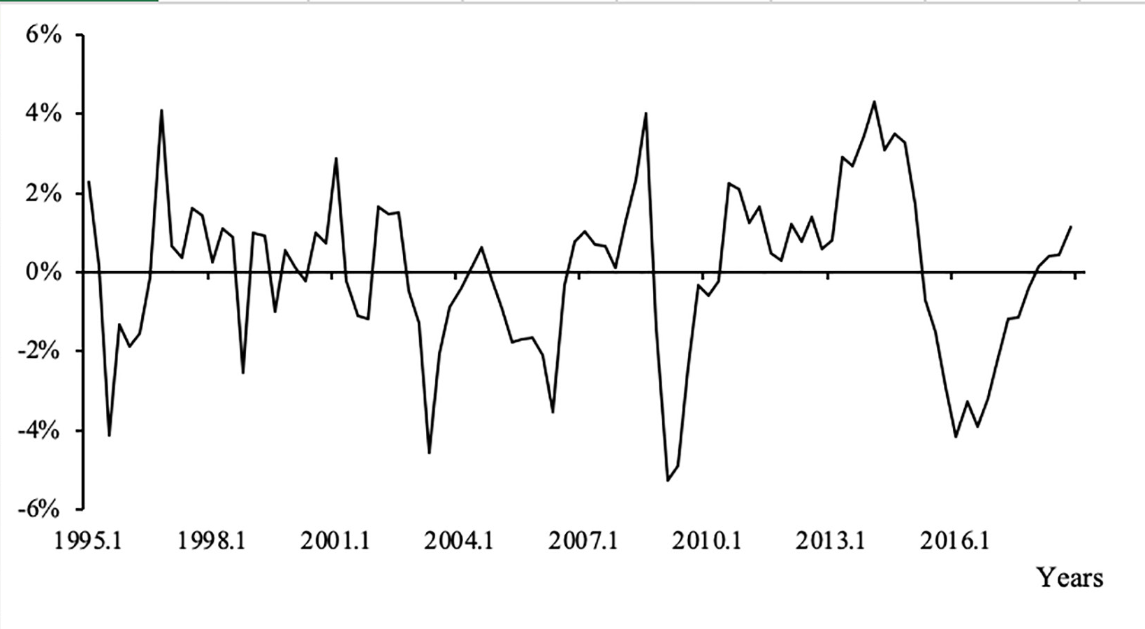
Figure 8
Brazil: GDP Cyclical Component
Source: Own estimates based on International Financial Statistics (IMF).

In fact, according to Souza-Sobrinho (2010), the 1995 recession stems from the Mexican crisis that extended its effects to almost all emerging markets. A similar situation occurred in 1998 due to the Russian crisis. The 2002-2003 recession is associated to the Argentine financial crisis and to uncertainties around the election of a left-wing president in Brazil. The 2008-2009 crisis was a consequence of the subprime international crisis, while the 2015-2016 one was due to the huge augment in the household debt aggressively promoted by public banks (Garber et al., 2019). During the last years, real GDP is nearly aligned with its declining trend.

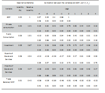
Table 2 shows the volatility and co-movements of the GDP components as well as their correlation coefficients¹⁵. The table shows that the volatility of the Brazilian economy is 2.05%. This volatility is less than that observed in Argentina probably due to better macroeconomic poli- cies implemented by Brazil.¹⁶ As in the case of Argentina, it is impor- tant to observe the volatility of other macroeconomic variables (abso- lute volatility) and to compare it with the volatility of GDP (relative volatility), as well as their phase shift.

Table 2

Brazil: Cyclical behavior of real GDP and its main components(1995.1-2018.4)

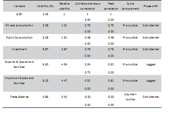
Source: Own estimates based on International Financial Statistics (IMF)

Figure 9 shows that volatility for private consumption is roughly the same than that for GDP, as expected, since this is a typical fact among developing countries. Private consumption exhibits a strong correlation (0.75) with GDP at the contemporaneous level, it acts pro-cyclically and similar results have been obtained by Kanczuk (2004) and Souza- Sobrinho (2011).

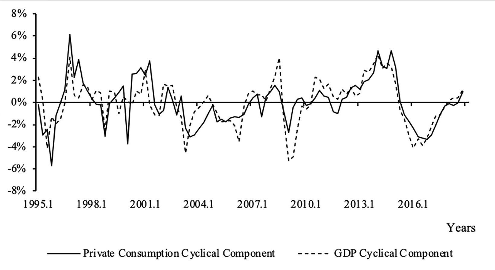
Figure 9
Brazil: GDP and Private Consumption cyclical components
Source: Own estimates based on International Financial Statistics (IMF)

This result is consistent with the findings of Ellery Jr., Gomes and Sachsida (2002), a little bit lower than the results of Souza-Sobrinho (2011), but higher than those obtained by Kanczuk (2004).

A similar pattern follows public consumption. Its cyclical component is drawn in Figure 10. It is correlated (0.48) and more volatile (50%) than GDP.

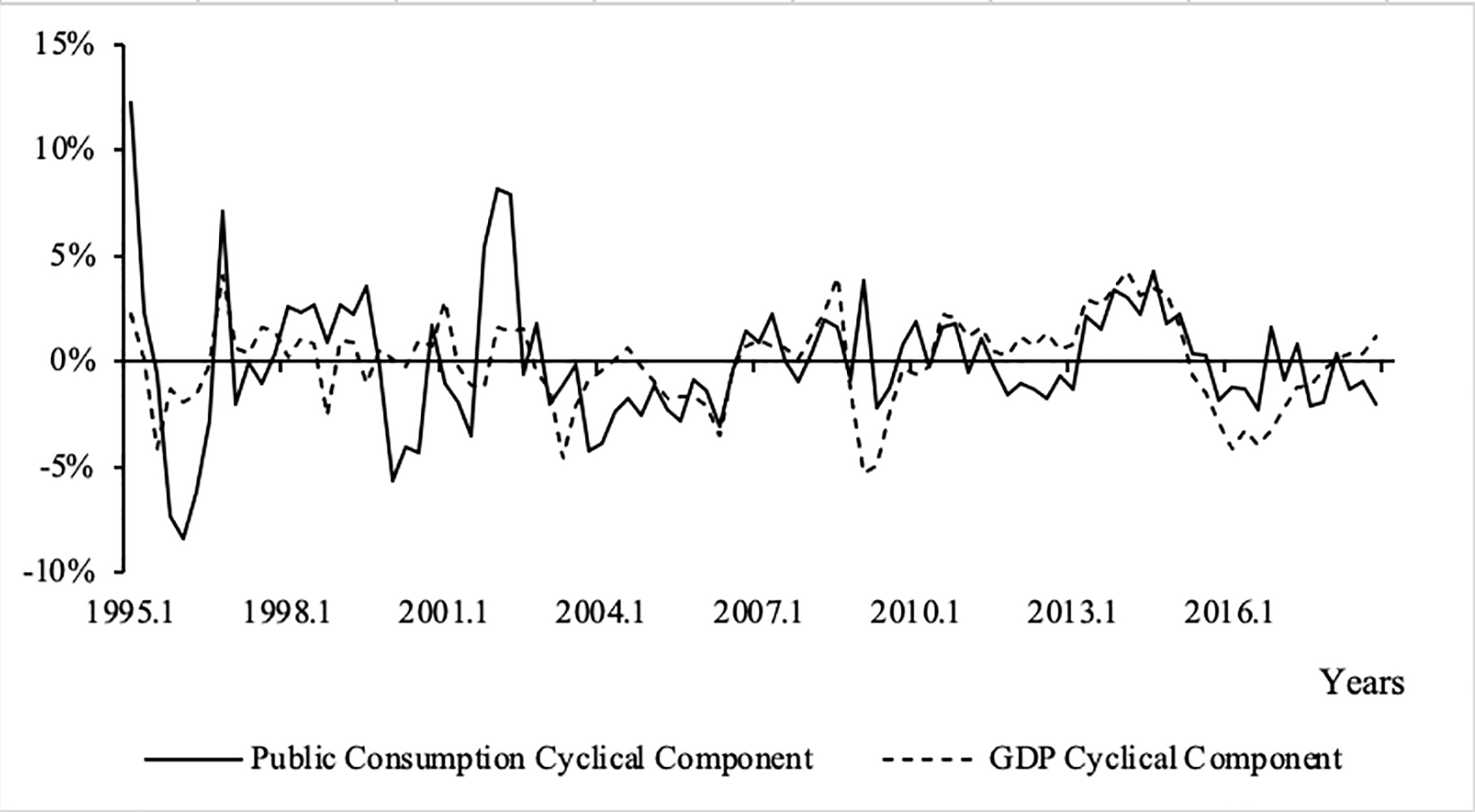
Figure 10
Brazil: GDP and Public Consumption cyclical components
Source: Own estimates based on International Financial Statistics (IMF)

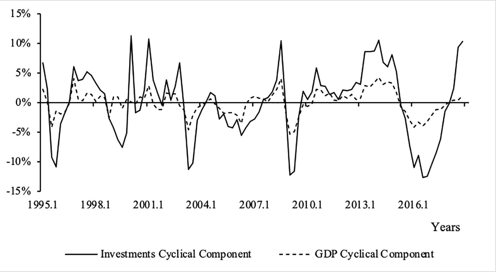
Figure 11
Brazil: GDP and Gross Investment cyclical components
Source: Own estimates based on International Financial Statistics (IMF).

Investment is much more volatile (2.8 times) than GDP and highly correlated with output (0.79). When contemporaneous variables are considered, the coefficient is the highest, as observed by Aguiar and Gopinath (2004), Val and Ferreira (2002), Ellery Jr., Gomes and Sachsida (2002), Neumeyer and Perri (2005), Souza-Sobrinho (2011) and Kanczuk (2004). This relation is represented in Figure 11.

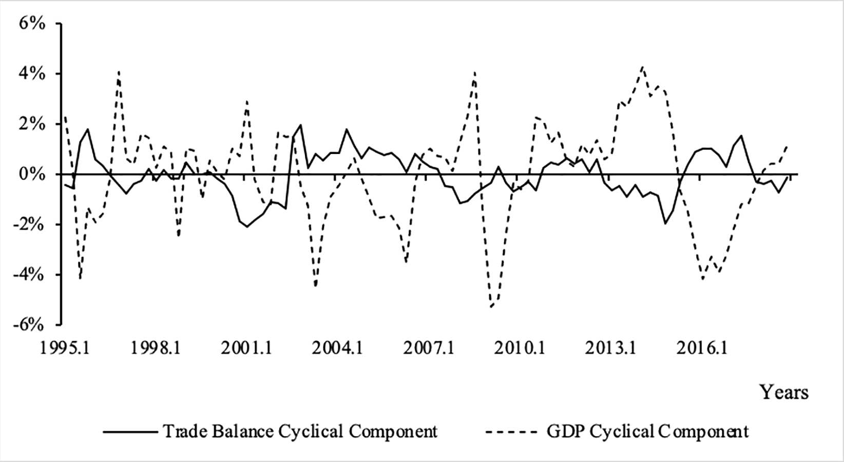
Figure 12
Brazil: GDP and Trade Balance cyclical components
Source: Own estimates based on International Financial Statistics (IMF)

Imports and exports are 4 times more volatile than GDP and significantly correlated with GDP, thus revealing a pro-cyclical pattern. While our results are consistent with Ellery, Gomes and Sachsida (2002), their measures are somewhat different. The exports are positively correlated with GDP for lagged values, but negatively correlated for future values. This may be a consequence of the different periods analyzed as well as different dynamics of the exports during devaluations.

Trade balance cycle is depicted in Figure 12. We find this variable to be less volatile than GDP and to act counter-cyclically and coincidentally. While Aguiar and Gopinath (2004) find that net exports are more volatile (probably due to the period analyzed), other studies find an a-cyclical and less volatile behavior as we do (Neumeyer and Perri, 2005; Souza-Sobrinho, 2011).

3.3. Argentina and Brazil: How close are they to each other?

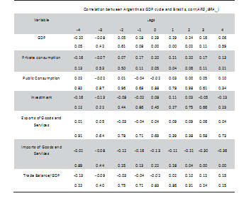
The purpose of this subsection is to illustrate the relation between the business cycles of Argentina and Brazil and to show the correlation between both cycles and their cyclical components. Figure 13 presents the evolution of the business cycle of Argentina and Brazil, and Table 3 summarizes some of our findings.

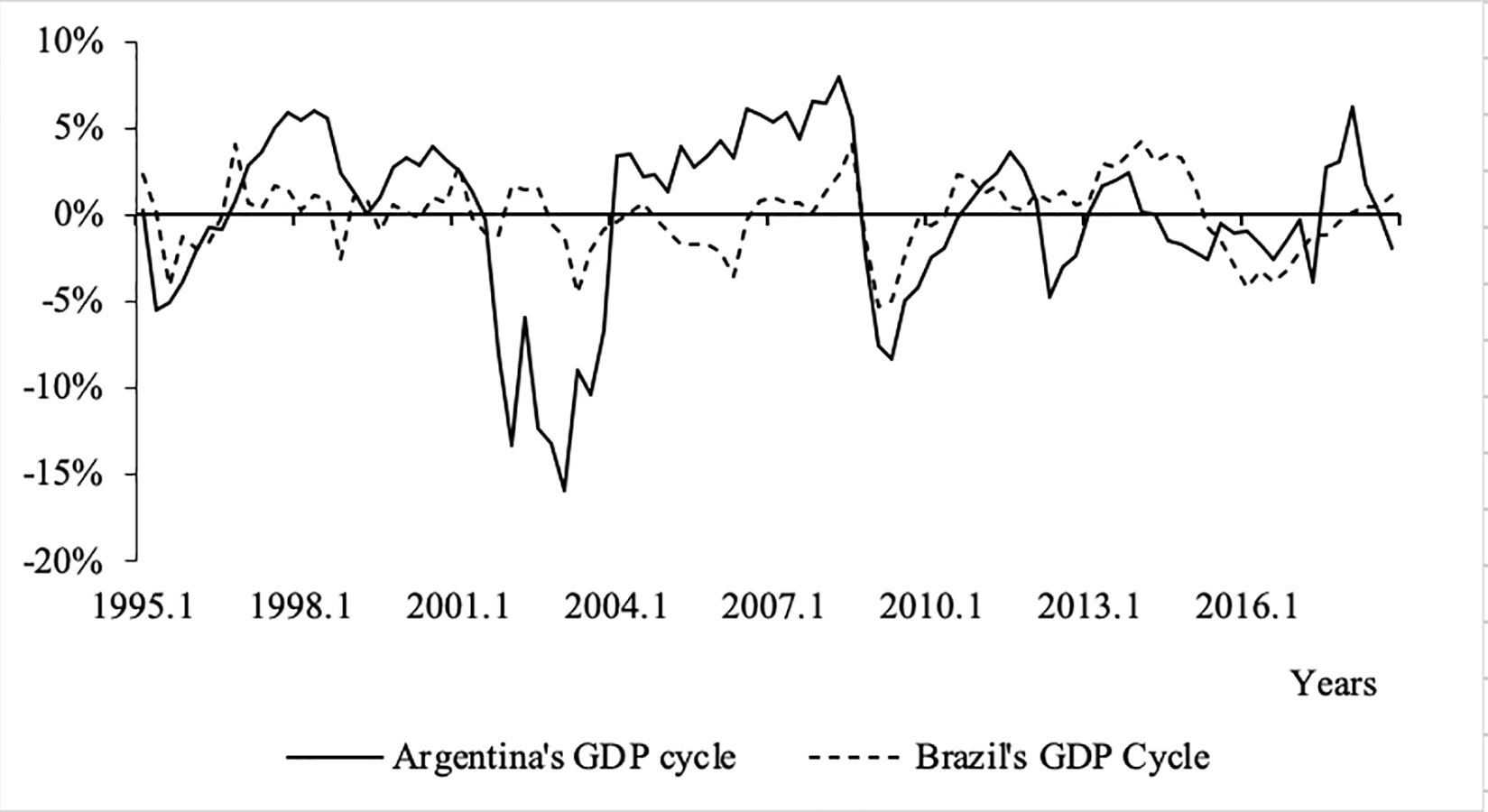
Figure 13
Business Cycles of Argentina and Brazil
Source: Own estimates based on International Financial Statistics (IMF)

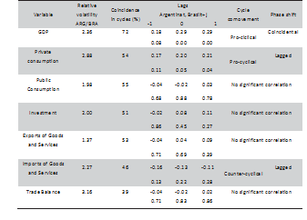
First, Argentina’s GDP cycles are sharper and longer than those of Brazil. According to our previous findings, it is not strange to find bigger standard deviations for Argentina than for Brazil. In fact, Argentinean GDP and all its components are more volatile than Brazilian variables: GDP is 2.36 times more subject to unexpected change, private consumption is nearly three times more instable (2.98), public consumption and investment are almost twice (1.98 and 2.00 respectively), and exports (1.37) and imports (2.27) also reflect more variability.

A plausible explanation about this goes beyond the extent of the paper. However, we claim that some of these findings can be reconciled with the theory of “stop-and-go” cycles based on a strong, contractio- nary devaluations and recoveries via expansive demand-driven policies.

According to Sturzenegger and Moya (2003), history shows that devaluations in Argentina were used to solve balance of payment problems through an increase in tradable prices that, in turn, caused a fall in real wages and in the real money supply. This policy of exchange rate deva luations was against all priors in that it was decidedly contractionary and not expansionary as in the Mundell-Fleming model.¹⁷

Table 3

Argentina and Brazil: Business cycles features

Source: Own estimates based on International Financial Statistics (IMF)

Second, if we consider the percentage of quarters over the total quarters analyzed in the sample when both cycles have the same sign (both positive or both negative), the highest coincidence is observed in GDP (72% of our observations of both variables are at the same side of the zero line). This means that whenever one country is undergoing a negative (or positive phase), the same is happening in the other country.

However, there is no deterministic order of this coincidences. As to the rest of the variables, the coincidences are also important (more than 50% of the observations lie at the same side of the zero): private and public consumption (54 and 55% respectively), investment (51%) and exports (53%). As to imports, the coincidences fall below 50% (the correspondence is 46%).

Third, the only Argentinian variables that has a significant correlation with its Brazilian counterpart are GDP, private consumption and imports, but these correlations are rather moderate. Brazil leads Argentina’s GDP cycle (it is one quarter ahead) with a coefficient of about 0.29, and it leads Argentina’s private consumption cycle (again, Brazil is one quarter ahead) with a coefficient of roughly 0.21. That is, Brazil’s GDP and private consumption acts pro-cyclically. As to imports, their cycle is lagged 4 quarters (-0.36) with the highest and statistically significant coefficient.¹⁸

Concluding remarks

The aim of this work is to provide some new features and stylized facts for GDP business fluctuations of Argentina and Brazil for the period 1995.1-2018.2. It is motivated by the lack of novel research on business cycles in these countries and by the importance of studying the synchronism of the cycles in the region.

According to our findings, Argentina’s GDP fluctuations are sharper and longer than those of Brazil. Additionally, GDP components are also more volatile in Argentina than in Brazil. Notwithstanding other causes may have influenced in this behavior, this probably means that Brazilian economy has had better macroeconomic policies than Argentina.

The main stylized facts clearly coincide in both economies. In fact, private and public consumption, as well as investment, tend to act pro- cyclically. Exports act a-cyclically and the trade balance tends to behave counter-cyclically. However, one must be cautious when interpreting these results because exports may become strongly pro-cyclically after a devaluation and before the pass-through mechanism.

When these economies are analyzed together, their business fluctuations have the same sign (both positive of both negative) and the highest coincidence is observed in GDP (72% of the observations in both variables are at the same side of the zero line). This means that whenever one country is undergoing a negative (or positive phase) the same is happening in the other. Nevertheless, as to the rest of the variables, the coincidences drop to nearly 50%. The only Argentinian variables that have significant correlations with its Brazilian counterpart are GDP, private consumption and imports, but these correlations are quite modest.

To sum up, since the nineties, deliberative efforts have been done to achieve a higher degree of trade and financial integration. As the economy has become more integrated, the interdependence has augmented and much of the world has moved in tandem. However, it seems not to be the case of Argentina and Brazil. Their business fluctuations are not at all uniform.

Although it is not the purpose of the paper to further analyze the causes of this situation, we suspect that the different political perspectives of party leaders have notably influenced on the dissimilar patterns we have observed. If this is the case, the countries will probably be better together as soon as their political leaders conceive a strategic and steady approach towards economic integration.

References

Agénor, C., McDermott, J. and S. Prasad (2000). “Macroeconomic Fluctua- tions in Developing Countries: Some Stylized Facts”, The World Bank Economic Review, 14 (2), pp. 251-285.

Aguiar, M., and G. Gopinath (2007). “Emerging market Business Cycles: The cycle is the trend”, Journal of Political Economy, 115, pp. 69-102.

Ahumada, H. and M. Garegnani (1999). “Hodrick-Prescott Filter in Practice”, paper presented at the V Jornadas de Economía Monetaria e Internacional.

Aiolfi, M., Catão, L. and A. Timmermann (2006). “Common Factors in La- tin America’s Business Cycles”, IMF Working Paper 06/49, International Monetary Fund.

Arnaudo, A. A. and A. D. Jacobo (1997). “Macroeconomic Homogeneity within MERCOSUR: An Overview”, Estudios Económicos, 12 (1) pp. 37- 51.

Baxter, M. and R. King (1995). “Measuring Business Cycles Approximate Band-Pass Filters for Economic Time Series”, National Bureau of Econo- mic Research Working Paper 5022.

Capello, M. and N. Grión (2003). “Ciclos Macroeconómicos y Fiscales en la Argentina de la Convertibilidad. Principales Hechos Estilizados”, ma- nuscrito, Departamento de Economía y Finanzas. Facultad de Ciencias Económicas. Universidad Nacional de Córdoba, 16. 1-24.

Catão, L. (2007). “Latin America Retrospective”, Finance and Development, 44 (4), pp. 39-43.

Cerro, A. and J. Pineda (2002). “Latin American Growth Cycles. Empirical Evidence 1960-2000”, Estudios de Economía, 29 (1), pp. 89-108

Cerro, A. (1999). “La Conducta Cíclica de la Economía Argentina y el Com- portamiento del Dinero en el Ciclo Económico Argentina 1820-1998”, Económica, 157 (3), pp. 8-60.

Christiano, L. and T. Fitzgerald (1999). “The Band Pass Filter”, National Bu- reau of Economic Research Working Paper 7257.

Cleveland, R. B., Cleveland, W. S., McRae, J. E., and I. Terpenning (1990). “STL: A Seasonal-Trend Decomposition Procedure Based on Loess”, Journal of Official Statistics, 6 (1), pp. 3-33.

Cogley, T. and J. Nason (1995). “Effects of the Hodrick-Prescott filter on trend and difference stationary time series Implications for business cycle re- search”, Journal of Economics Dynamics and Control, 19 (1-2), pp. 253- 278.

DeLong, J. and L. Summers (1986). “Are Business Cycles Symmetrical?”, in R. J. Gordon, The American Business Cycle: Continuity and Change. Uni- versity of Chicago Press for the National Bureau of Economic Research, Chicago, pp. 166-178.

Díaz, C. (2007). “Characterization of the Argentine Business Cycle”, manus- cript, Universidad Carlos III de Madrid, Madrid.

Ellery Jr., R., Gomes, V. and A. Sachsida (2002). “Business Cycle Fluctuations in Brazil”, Revista Brasileira de Economia, 56 (2), pp. 269-308.

Arbatli, E. C. (2009). “Business Cycle in Emerging Economies: Sudden Stop and the Cycle”, in E. C. Arbatli: Persistence of Income shock and the In- tertemporal Model of Current Account. Johns Hopkins University, Balti- more, pp. 92-132.

Enders, W. (1995). Applied Econometric Time Series. John Wiley & Sons, New York.

Engle, R. F. and J. Issler (1993). “Common Trends and Common Cycles in Latin America”, Revista Brasileira de Economia, 47 (2), pp. 149-176.

Frankel, J. A., Vegh, C. A. and C. Vuletin, G. (2011). “On graduation from fiscal procyclicality”, Journal of Development Economics, 100 (1), pp. 32-47.

Frankel, J. and A. Rose (1998). “The Endogeneity of the Optimum Currency Area Criteria”, The Economic Journal, 108(449), 1009-1025.

Garber, G., Mian, A., Ponticelli, J. and Sufi (2019). “Household debt and re- cession in Brazil”, in A. Haughwout and B. Mandel Handbook of US Con- sumer Economics. San Diego: Academic Press, San Diego, pp. 97-119.

Gutierrez, C. and F. Gomes (2009). “Evidence on Common Features and Busi- ness Cycle Synchronization in Mercosur”, Brazilian Review of Econometrics, 29 (1), pp. 37-58.

Gonzalez, G. H. and A. M. Patiño (2012). “Sincronización de Ciclos e Inte- gración Latinoamericana: nuevas hipótesis tras otro ejercicio empírico”, Trayectorias, 14 (35), pp. 3-26.

Hamilton, J. D. (2017). “Why you should never use the Hodrick-Prescott Filter”, National Bureau of Economic Research Working Paper 23429.

Hamilton, J. D. (1989). “A new Approach to the Economic Analysis of Nons- tationary Time Series and the Business Cycles”, Econometrica, 57 (2), pp357-384.

Harvey, A. and A. Jeager (1993). “Detrending, Stylized Facts and the Business Cycle”, Journal of Applied Econometrics, 8 (3), pp. 231-247.

Jacobo, A. (2002). “Taking the business cycle´s pulse to some Latin American economies: Is there a rhythmical beat?”, Estudios Económicos, 17 (2), pp. 219-245.

Jorrat, J. M. (2005). “Construcción de índices compuestos mensuales coincidente y líder en de Argentina”, in M. Marchioni (Ed.) Progresos en Econometría, Series Progresos en Economía, Asociación Argentina de Economía Política, Argentina.

Kanczuk, F. (2004). “Real Interest Rates and Brazilian Business Cycles”, Re- view of Economic Dynamics, 7 (2), pp. 436-455.

Kydland, F. E. and E. C. Prescott (1990). “Business Cycles: Real Facts and a Monetary Myth”. Federal Reserve Bank of Minneapolis Quarterly Re- view, 14, pp. 3-18.

Kydland, F. E. and C. E. Zarazaga (1997). “Is the Business Cycle of Argentina “Different”?”, Federal Reserve Bank of Dallas Economic Review, fourth quarter, pp. 21-36.

Loayza, N., Fajnzylber, P. and C. Calderón (2004). “Economic Growth in Latin America and the Caribbean: stylized facts, explanations and forecasts”, Banco Central de Chile Working Paper 265.

Lucas, R. E. (1977). “Understanding Business Cycles”, Carnegie-Rochester Conference Series on Public Policy. Elsevier B.V., The Netherlands, 7-29.

Mejía, Pablo. (1999). “Classical business in Latin America: turning points, as- ymmetries and international synchronization”, Estudios Económicos. 14, (2), pp. 265-297.

Neumeyer, P. A. and F. Perri (2005). “Business Cycles in Emerging Econo- mies: The Role of Interest Rates”, Journal of Monetary Economics, 52 (2), pp. 345-380.

Ravn, M. and H. Uhlig (2001). “On Adjusting the HP-Filter for the Frequency of Observations”, CEPR Discussion Paper 2858.

Rojas, M., Zilio, M. and S. Zubimendi. (2009). “Hechos Estilizados para la Economía Argentina”, Ensayos Económicos, 56, pp. 157-210.

Söderlin, P. (1994). “Cyclical Properties of a Real Business Cycle Model”, Applied Econometrics, 9 (S1), pp. 113-122.

Souza-Sobrinho, N. F. (2010). “The Role of Interest Rates in the Brazilian Business Cycle”, Revista Brasileira de Economia, 65 (3), pp. 315-336.

Srivastava, U., G. Shenoy and S. Sharma (2005). Quantitative Techniques for Managerial Decisions. Concepts. Illustrations and Problems, New Age International Ltd. Publishers, Dheli.

Sturzenegger, A. and R. Moya (2003). “Economic Cycles”, in G. della Paolera and A. Taylor A (Ed.) New Economic History of Argentina, Cambridge University Press, United States.

Toledo, M. (2008). “Understanding Business Cycles in Latin America”, manuscript, Universidad Carlos III de Madrid, Madrid.

Val, P. R. and Ferreira, P. C. (2002). “Modelos de Ciclos Reais de Negócios Aplicados á Economia Brasileira. Ensaios Economicos, 438, pp. 215-248.

Appendix A

Table A.1

Argentina: Cyclical behavior of GDP and its components (1995.1-2018.4)

Correlation coefficients correspond to Spearman’s rank-based statistic.

Table A.2

Brazil: Cyclical behavior of GDP and ist components (1995.1-2018.4)

Correlation coefficients correspond to Spearman’s rank-based statistic.

Table A.3

Argentina and Brazil: Association between their business cycles and GDP (1995.1-2018.4)

Correlation coefficients correspond to Spearman’s rank-based statistic.

Notes

Author notes