1. INTRODUCTION

The Ground Penetrating Radar (GPR) provides an accurate and non destructive solution for estimating the subsurface electromagnetic parameters through the propagation of electromagnetic waves [1]. GPR systems provide real-time analysis, allowing users to safely identify features and objects before drilling or trenching, in such manner that environmental hazards can be avoided.

With the acquired data, the electromagnetic characteristics of the soil (e.g., permittivity, permeability, and conductivity) can be estimated via Full Waveform Inversion (FWI). FWI is an iterative local optimization method that uses a cost function to minimize a distance between the observed data (measured in the field) and the modelled data (obtained by simulation). FWI requires an initial model of subsurface parameters with enough low-wavenumber information, and the signature of the source used during the data acquisition process. Those requirements enable the accurate reconstruction of the underground parameters in FWI. [2]. Including the radiation properties of the antenna in the wave modelling also provides simulated data that resembles the observed data.

Different methods have been used to estimate the source signature for FWI, such as the characterization of the antenna as an infinitesimal dipole, where the energy in TE mode is distributed uniformly for any angle [3], or the signature estimation from the acquired data using the adjoint state method [4], the variable projection method [5], [6] and gradient-based optimization methods [7]. Other proposed methods are reverse-time propagation [8], and the deconvolution of radar data with the parameters system [9].

In this paper, the source signature is obtained by estimating the internal electromagnetic parameters of the GSSI shielded antenna. The parameter estimation problem is formulated as a global optimization issue that compares the simulated electric field (R_xmod) with the measured electric field (R_xobs) for a set of possible parameter values. The inverse problem is solved using a global optimization algorithm called Particle Swarm Optimization (PSO). This method generates particles with the possible values for the internal parameters of the antenna at random in a predefined search space [10]. The global optimization algorithm compares R_xobs and R_xmod using two metrics: one in time domain, and the other in frequency domain. The antenna used in this study is a commercial GSSI brand GPR with an operating frequency of 400 [MHz]. The antenna's pattern that describes the energy radiation out into the ground is obtained from the estimated internal parameters of the antenna. Such radiation pattern is then included in the electromagnetic wave propagation and the inversion process.

The soil parameter model used in this paper to test the inversion process is the SEG Advanced Modelling (SEAM) Foothills model [11]. This model was inspired by the Andes mountains in Colombia with compressive tectonics [11].

This paper is divided in four sections. The theoretical framework for both inverse problems: the antenna parameters and FWI, is presented in the first section. Then, a methodology for the estimation of the internal parameters of the antenna and its use in FWI is presented. The next section shows the experimental results of the commercial GSSI antenna characterization, and the estimation of the soil parameters. Finally, the last section gives a brief discussion and conclusions on the proposed methods.

2. THEORETICAL FRAMEWORK

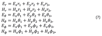
A GPR system mainly consists of three instruments: the control unit, a display system, and the transmitter (Tx) and receiver (Rx) antennas [12]. The commercial system, designed and built by the GSSI at 400 [MHz], is shielded and the Tx-Rx antennas have a single-channel and short-offset configuration. The shielded system is used in GPR applications where the distance between both Tx and Rx antennas is fixed. The internal geometry of a shielded antenna is depicted in Figure 1. The parameters W, L, and h are 6 [cm]. The distance between both antennas, known as the offset, is 16.2 [cm]. The electromagnetic pulse generated by the antenna, considering the internal geometry and its electromagnetic properties, is modelled using the gprMax commercial software [13].

Figure 1
Internal geometry of the shielded GSSI antenna at 400 [MHz].

The estimation of the electromagnetic properties of the antenna is based on the workflow shown in Figure 2. An electric field is measured at the receiver antenna, and it is called R_xobs. A simulated electric field is obtained using the gprMax commercial software, and it is called R_xmod [14]. The simulated electric field at the receiver antenna, is a function of the electromagnetic parameters of the antenna: the relative permittivity of the absorbent barrier, ε_r(abs); the relative conductivity of the absorbent barrier, σ_r(abs); the relative permittivity of the Printed Circuit Board (PCB), ε_r (PCB); the relative permittivity of the housing, ε_r (housing); and the Tx and Rx resistance.

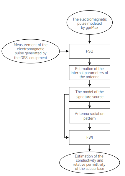
Figure 2
Methodology for the estimation of the internal parameters of the shielded antenna.

The gprMax software simulates the wave propagation of the source, based on the discretized version of the following time domain wave equations,

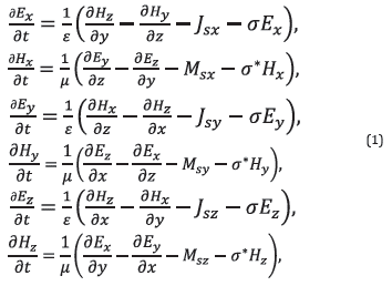
where ε, σ, μ are the permittivity [F/m], permeability [H/m] and conductivity [S/m], respectively; σ^* is the equivalent magnetic loss [Ω/m]; E_x, E_y, E_z are the electric fields in the direction x, y and z, respectively; H_x, H_y, H_z are the magnetic fields in the direction x, y and z respectively; J_sx, J_sy and J_sz are the densities of electric current at x, y and z, respectively; and M_sx, M_sy, M_sz are the magnetic current densities at x, y and z, respectively [15]. In all experiments μ=1 since the materials are not magnetic, and σ^*=0 because the magnetic losses are zero. On the other hand, the excitation and reception of the electric current density is only applied in the y-direction due to the orientation of the antennas; therefore J_sx =0 and J_sz =0.

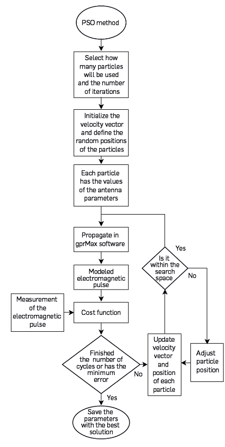
Figure 2
PSO inversion process to estimate the internal antenna parameters.

The Particle Swarm Global Optimization (PSO) method seeks the best combination of the internal parameters to minimize a given cost function (see Figure 3). In this paper, two metrics are proposed to measure the similarity between the measured electric field R_xmod and the simulated electric field R_xmod. First, the cross-correlation in time domain is used [16]. The cross-correlation equation is given by,

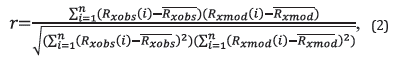
where () and () are the mean value of R_xobs and R_xmod1 respectively.

A second metric that measures the difference of the maximum values of the amplitude spectrum of R_xobs and R_xmod, is used in the global optimization method. This is given by,

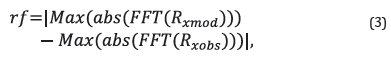
where |∙| is the modulus, Max(∙) is the maximum value, abs(∙) is the amplitude spectrum and FFT(∙) is the Fast Fourier Transform.

PSO is an iterative method that randomly creates a group of particles, where each particle contains the information of each antenna parameter (see Figure 1). All the particles keep the memory of their best position vector and their velocity vector [17]. In each iteration, a particle velocity adjustment is made, according to the best previous position occupied by the particle (i) and the best position of the group of particles, as it is given by,

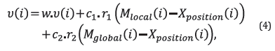
where w=0.3, c₁=0.5 and c₂=2.05 are constants of each optimization problem; r₁ and r₂ are random values between 0 and 1; X_position is the current position of the particle; M_global is the best position of the particle group; and M_local is the best position previously occupied by the particle. The position vector is updated with the current position and the new velocity vector as,

This process is iterative, and it stops when it reaches several iterations or until a minimum error value is obtained. Once the antenna parameters are estimated, its radiation pattern can be obtained. The radiation patterns give the distribution of the energy in the subsurface [3].

One of the challenges addressed in this paper is the estimation of the radiation patterns for a shielded antenna with a fixed offset. The radiation pattern is measured in a spherical coordinate system as shown in FIGURE 4. The radiation pattern is transformed from spherical coordinates to cartesian coordinates such that the electric and magnetic fields can be obtained for each time. For the transform of the coordinates, x, y, and z are defined as: x=rcos(φ) sin(θ) , y=rsin(φ)sin(θ), and z=rcos(θ). The transformed points from spherical to cartesian coordinates are not exact values on the mesh thus requiring an interpolation. In this case, a bilinear interpolation is performed for a given value f(x,z), with xand z being the locations in distance-direction and depth-direction, respectively [18].

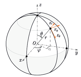
Figure 4
Spherical coordinate system used to transform the radiation pattern to rectangular coordinates.

The pattern radiation generated by the source of the GSSI antenna can be estimated in spherical coordinates by,

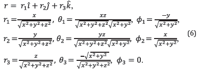
The electric field in terms of r, θ and ϕ are defined as,

The sum of all the squared values of E_θ and H_θ are computed to obtain the radiation plane E and H, respectively. The energy for each plane is given by,

FULL WAVEFORM INVERSION

The inverse problem estimates the soil parameters m(ε_r ,μ_r , σ_r ) from the observations on surface R_xobs , the electric field E_y and a known source (J_s ). Full Waveform Inversion (FWI) minimizes the l² - norm squared of the difference between the modeled data R_xmod(m^k) and R_xobs observed data [19], as follows

With

where m^k are the unknown parameters in the k-th iteration, Ns the number of sources, R is the operator that extracts the electromagnetic wavefield E_y at the receiver positions and s is the electromagnetic vector fields [E_y, H_x, H_z]. The inverse problem can be solved iteratively by selecting an initial parameters model m⁰, and updating it by using Newton-like methods [20], as

where α_k is the step size and Δm^k at the k^th iteration is given by

The inverse of the Hessian matrix [h(m^k)]^-1 and the gradient g(mk), in the Equation (12) are both evaluated at m^k [21]. As the inverse problem is ill-posed, the cost function given in Equation (9) has several minimums and an inadequate starting point (m⁰ ) will produce convergence to a local minimum.

The electromagnetic wave equations in a non-dispersive and isotropic medium are considered where the fields E_y , H_x and H_z are different from zero. The forward operator is described by

where σ_r is the relative conductivity; this relative parameter is a scale setting for the conductivity value, where σ₀ is an arbitrary scale value. The expression for σ_r is as follows σ_r=σ/σ₀; ε_r is the relative permittivity; ε₀ and μ₀ are the permittivity and permeability in the vacuum, respectively. For all the experiments, ε₀≅8.85 . 10^-12, μ₀ ≅4π .10^-7 and σ0=5.56.10^-4.

On the other hand, the adjoint operator for the cost function is defined as

where ∂Φ/∂s=R_xmod(s)-R_xobs . Also, λ_Ey, λ_Hx , and λ_Hz are the adjoint fields for E_y , H_x and H_z , respectively. The following expressions are defined to obtain the gradients for permittivity and conductivity.

3. RESULTS AND ANALYSIS

ESTIMATION OF THE ANTENNA INTERNAL PARAMETERS

The results of the antenna parameters estimation are presented in this section. For the PSO method, a total of 65 experiments were performed. The searching regions for the source and receiver resistance (r) ranges between [1-1000] [Ω]; for εr(abs), ε_r (housing) and ε_r (PCB) range between [1-30] [F/m]; and finally, for σ_r (abs) ranges between [0-20] [S/m]. The sample space for all parameters within the searching region is 1x10^-5.

The materials of the internal structure of the antenna estimated with the proposed method were r= 49.22 [Ω], ε_r (abs)=3.89, σ_r (abs)=0.02 [S/m], ε_r (PCB) =7.44 [F/m], and ε_r (hdp) = 1.00 [F/m]. The error between R_xobs and R_xmod using the estimated parameters is 2.65%. Figure 5-a) and 5-b) show the resulting signals in time and frequency, respectively.

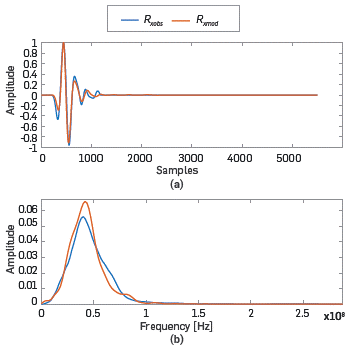
Figure 5
a) Rxmod and Rxobs in the time domain. b) Frequency spectrum for Rxmod and Rxobs.

The bowtie antenna can be represented using a dipole as an approximation. For the case of an y-axis oriented dipole, the radiation pattern will be a toroid as shown in Figure 6-a) and their respective views in the x-z and y-z planes are presented in Figure 6-b) and c), respectively.

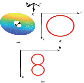
Figure 6
Radiation patterns for an oriented dipole: a) 3D view, b) plane x-z and c) y-z.

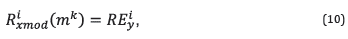
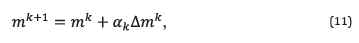
The electric and magnetic fields are measured at a radius from 0.2 [m] to 0.9 [m] and a dr = 0.12 [m]. The angle of observation ranges from 0 [rad] to 2π [rad] with dθ = 0.104 [rad]. The results, in Figure 7, show the radiation patterns in two-dimensions. However, given the antenna’s internal geometry, the energy is attenuated between -60° and 60°. The resulting radiation patterns are included in the propagation of the electromagnetic field, and in the inverse problem. The radiation pattern in cartesian coordinates is shown in Figure 8-a) and 8-c) for two different angles of the slope, but only the radius lower than 0.2 [m] is used in the wave propagation (see Figure 8-b) and 8-d)). The angle of the slope is required due to the rough topography of the SEAM model.

Figure 7
E and H planes of radiation for the shielded antenna at 400 [MHz]. a) and b) show the radiation patterns in polar coordinates (r [dB] vs θ [grades]) for planes E and H, respectively. The radius ranges from 0.2 [m] to 0.9 [m] with a step size of 0.116 [m]. c) and d) show the normalized radiation patterns with respect to the maximum value in planes E and H, respectively

Figure 8
Radiation patterns: a) with an angle of 0° of inclination, b) radiation pattern for a radius less than 0.2 [m] and 0° of inclination, c) with an angle of 39.78° of inclination, d) radiation pattern for radius less than 0.2 [m] and 39.78° of inclination.

FULL WAVEFORM INVERSION

This section presents the results of estimating the electromagnetic parameters of the source using the estimated source (J_s) and its radiation pattern (P_r). The radiation pattern is included in the wave propagation modelling by multiplying the pattern with the fields E_y, H_x, and H_z, where the electromagnetic equations are those for a non-dispersive and isotropic medium with and .

Experiment description: We use the previously estimated radiation pattern of the antenna to simulate the acquisition of GRP data from a single-offset antenna on the surface. The simulated observations are obtained supposing that the source has three different central frequencies: 30 [Mhz], 50 [MHz] and 100 [MHz]. For the wave propagation of the source with a central frequency of 100 [MHz] using the SEAM model, the spatial step in both dimensions is set to 0.05 [m], the time step is 0.06 [ns], and the total number of time samples is 3000 [10]. The model has 30 [m] in distance and 15.05 [m] in depth. The number of sources is 260 and they are equally distributed at 25 [cm] at the surface. The receiving antenna is located at 15 [cm] from the surface.

Figure 9-a), 9-b) and 9-c) show the wave propagation at the 500th time sample, and Figure 9-c), 9-d) and 9-f) present the wave propagation at the 1000th time sample. Figure 9-a) and 9-d) show the propagation including the radiation pattern at 0° of inclination. Figure 9-b) and 9-e) depict the propagation without considering the radiation pattern, and Figure 9-c) and 9-f) depict the propagation including an angle of inclination of 39.78° due to the slope of the rough topography. Notice at the red ovals in the Figure 9-a), 9-b) and 9-c) that the airwave energy distribution changes when the radiation pattern is included.

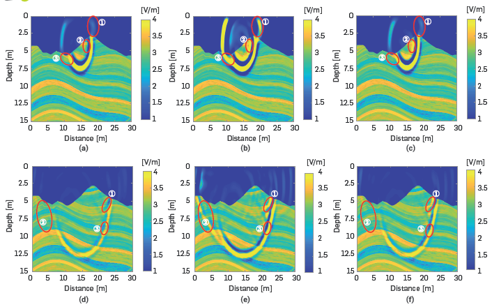
Figure 9
Propagation of the electromagnetic wavefront. First row: 500th time sample. Second row: 1000th time sample. a) Including the radiation pattern at 0° of inclination, b) without radiation pattern, c) including the radiation pattern at 39.78° of inclination.

The reconstruction of the electromagnetic properties of the SEAM model is studied for three different scenarios: 1) The SEAM model has a rough topography, and the initial model is a smooth version of the original model. 2) The SEAM model has a rough topography, and the initial model is a constant value. 3) The SEAM model has a flat topography, and the initial model is a smooth version of the original model. The proposed tests seek to study the effects of topography in the model and the initial models for permittivity and conductivity.

Figures 10, 11, and 12 show the estimated models for the three proposed scenarios. In all tests, 30 iterations are performed for each central frequency of the source. The first row in Figures 10, 11 and 12, is the relative permittivity parameter, and the second row is the relative conductivity parameter. Further, the first column presents the original models; the second column shows the initial models; the third column gives the FWI results obtained using the radiation pattern, and the last column shows the results of FWI, not including the radiation pattern.

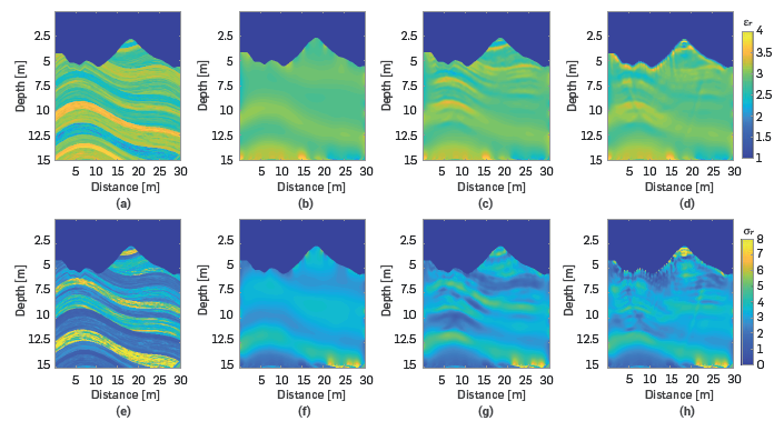
Figure 10
FWI results considering the radiation pattern. The first row is the relative conductivity, and the second row is the relative permittivity. a) and e) original models, b) and f) initial models, c) and g) models obtained after FWI multi-scale using the radiation pattern and d) and h) models obtained after FWI multi-scale without the radiation pattern.

The Peak Signal to Noise Ratio (PSNR) is used as quantitative error measurement between the ground real image and the estimated images. The PSNR for the initial models are 24.29 [dB] for permittivity and 24.56 [dB] for conductivity. When the radiation pattern is included, the resulting images reach PSNR values of 25.66 [dB] for relative permittivity (see Figure 10-c)) and 25.59 [dB] for conductivity (see Figure 10-g)). On the other hand, the images obtained when the radiation pattern is not included reach a PSNR of 23.69 [dB] for permittivity (see Figure 10-d)), and 22.87 [dB] for conductivity (see Figure 10-h)).

Figure 11 shows the estimated models when uniform initial models are used. The initial model has constant values of relative permittivity of ε_r=3 and relative conductivity of σ_r=2.28. Visually, the images when the radiation pattern is included (see Figure 11-c) and g)) are slightly better than when the radiation pattern is not included (see Figure 11-d) and h)). Note in Figure 11-c) and 11-g) that the first layers of the SEAM model can be observed whereas, if the radiation pattern is not adequately included, then the solution produces artifacts in the shallow area in both parameters, which lead to erroneous visual interpretations. Nonetheless, the quantitative PSNR values are very similar in both cases; when the radiation patterns are included, the estimated model has PSNR values of 13.85 [dB] for the relative permittivity and 21.24 [dB] for the relative conductivity, and when the radiation pattern is not included, the PSNR values are 13.77 [dB] and 21.37 [dB] for relative permittivity and relative conductivity, respectively.

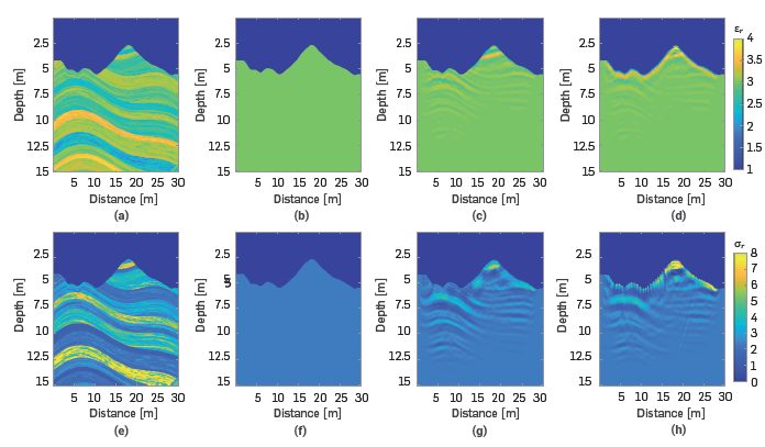
Figure 11
Estimated electromagnetic models using FWI. First row: relative permittivity. Second row: relative conductivity. a) and e) original models, b) and f) uniform initial models, c) and g) models obtained when the radiation pattern is included; and d) and h) models obtained when the radiation pattern is not included.

Figure 12 shows the estimated electromagnetic models when the topography of the SEAM model is flat. Note that for this experiment, the rough topography is not considered, but the antenna radiation pattern has an angle of inclination of 0 degrees. Figure 12-c) and 12-g) show a good quality image when the radiation pattern is included and the PSNR values are 26.52 [dB] for the relative permittivity and 26.19 [dB] for the relative conductivity. When the radiation pattern is not included, there are artifact effects on the near surface layer, which result in low quality imaging. The PSNR values for these images are 23.91 [dB] for the relative permittivity, and 23.69 [dB] for the relative conductivity.

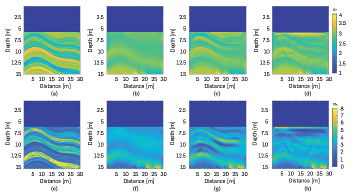
Figure 12
Estimated electromagnetic models using FWI. First row: relative permittivity. Second row: relative conductivity. a) and e) original models, b) and f) initial models, c) and g) models obtained when the radiation pattern is included; and d) and h) models obtained when the radiation pattern is not included.

Finally, Figure 13 depicts the error function for the three different scenarios studied in this paper. Note in this figure that the error is always less when the radiation pattern is included in the source wave propagation. Also, since the central frequency of the source changes every 30 iterations, the error increases at iterations 31 and 61, and then decreases again. This behaviour is equal in all experiments. The figure on the left depicts the cost function when the SEAM model has a rough topography, and the initial model is a smooth version of the original model. The figure in the middle is the cost function when the SEAM model has a rough topography, and the initial model is a constant value. Lastly, the image on the right is the cost function when the SEAM model has a flat topography, and the initial model is a smooth version of the original model.

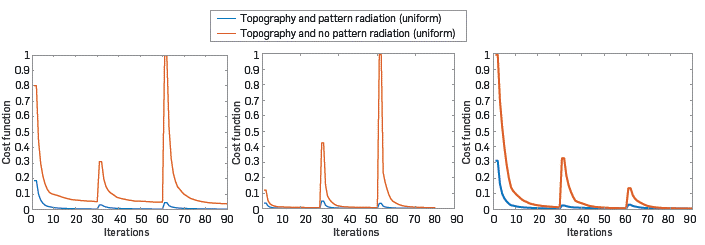
Figure 13
Error functions for three different scenarios. Left: the SEAM model has a rough topography, and the initial model is a smooth version of the original model. Middle: the SEAM model has a rough topography, and the initial model is a constant value. Right: the SEAM model has a flat topography, and the initial model is a smooth version of the original model.

CONCLUSIONS AND DISCUSSION

In this work, a global optimization method is proposed to find the internal physical parameters of a shielded antenna. The search for the best solution is based on two metrics: the maximum correlation between the observed and modelled signals, and the minimum difference of the spectrum amplitudes of the observed and modelled signals. The estimated parameters of the antenna are used to generate the antenna radiation pattern, which is used to simulate the wave propagation of a source throughout the SEAM synthetic model. Three different scenarios for the reconstruction of the ground electromagnetic parameters were evaluated: first, when the SEAM model has a rough topography, and the initial model is a smooth version of the original model; second, when the SEAM model has a rough topography, and the initial model is a constant value; and third, when the SEAM model has a flat topography, and the initial model is a smooth version of the original model

In sum, characterizing the source signal and including the correct radiation pattern in the synthetic inversion experiments was found to help inversion to converge to better quality images, either with flat or rough topography. The difference between the reconstructed images with radiation pattern and without radiation pattern is approximated 3 [dB] when the initial model is a smooth version of the correct solution.

When the initial model is constant, there is no significant difference in imaging when adding the radiation pattern. Hence, including the radiation pattern does not improve the solution if there is a poor starting model, as they do not provide enough low wavenumber information of the solution and, thus, reaching the correct solution would not be possible for FWI.

ACKNOWLEDGEMENTS

This research was sponsored by the Army Research Office and accomplished under Grant Number W911NF-17-1-0530. The views and conclusions contained in this document are those of the authors, and should not be interpreted as representing the official policies, either expressed or implied, of the Army Research Office or the U.S. Government. The U.S. Government is authorized to reproduce and distribute reprints for Government purposes notwithstanding any copyright notation herein. The authors gratefully acknowledge the support of CPS research group of Industrial University of Santander and Ecopetrol S.A.

REFERENCES

Daniels, D. J. (2004). Ground penetrating radar. 2nd ed. London, United Kingdom: The institution of Electrical Engineers. doi: https://doi.org/10.1049/PBRA015E

Lavoue, F., R. Brossier, L. Metivier, S. Garambois, and J. Virieux. (2014). Two-dimensional permittivity and conductivity imaging by full waveform inversion of multioffset GPR data: A frequency-domain quasi-Newton approach, Geophys. J. Int., 197(1), 248-268. doi: https://doi.org/10.1093/gji/ggt528

Diamanti, N. and A. P. Annan. (2013). Characterizing the energy distribution around GPR antennas, J. Appl. Geophys., 99, 83-90. doi: https://doi.org/10.1016/j.jappgeo.2013.08.001

Plessix, R. E. (2006). A review of the adjoint-state method for computing the gradient of a functional with geophysical applications, Geophys. J. Int ., 167(2), 495-503. doi: https://doi.org/10.1111/j.1365-246X.2006.02978.x

Golub, G. and V. Pereyra. (2003). Separable nonlinear least squares: The variable projection method and its applications, Inverse Probl., 19(2). doi: https://doi.org/10.1088/0266-5611/19/2/201

Fang, Z., R. Wang, and F. J. Herrmann. (2018). Source estimation for wavefield-reconstruction inversion, Geophysics, 83(4), R345-R359. doi: https://doi.org/10.1190/geo2017-0700.1

Liu, J., A. Abubakar, T. M. Habashy, D. Alumbaugh, E. Nichols, and G. Gao. (2018). Nonlinear inversión approaches for cross-well electromagnetic data collected in cased-wells, 78th Soc. Explor. Geophys. Int. Expo. Annu. Meet. SEG 2008, 1, 304-308. doi: https://doi.org/10.1190/1.3054810

Zhang, P., R. Gao, L. Han, and Z. Lu. (2021). Refraction waves full waveform inversion of deep reflection seismic profiles in the central part of Lhasa Terrane, Tectonophysics, 803(September 2020), 228761. doi: https://doi.org/10.1016/j.tecto.2021.228761

Ernst, J. R., A. G. Green, H. Maurer, and K. Holliger. (2007). Application of a new 2D time-domain fullwaveform inversion scheme to crosshole radar data, Geophysics, 72(5). doi: https://doi.org/10.1190/1.2761848

Russell, E. and S. Yuhui. (2001). Particle swarm optimization: Developments, applications and resources., Inst. Electr. Electron. Eng., 1, 81-86. doi: http://dx.doi.org/10.1109/CEC.2001.934374

Regone, C., J. Stefani, P. Wang, C. Gerea, G. Gonzalez, and M. Oristaglio. (2017). Geologic model building in SEAM Phase II-Land seismic challenges, Lead. Edge, 36(9), 738-749. doi: https://doi.org/10.1190/tle36090738.1

Jol, H. M. (2009). Ground penetrating radar : theory and applications, 1st ed. Amsterdam, The Netherlands: Elsevier B.V. doi: https://doi.org/10.1016/B978-0-444-53348-7.00017-X

Stadler, S. and J. Igel. (2018). A numerical study on using guided GPR waves along metallic cylinders in boreholes for permittivity sounding, 2018 17th Int.Conf. Gr. Penetrating Radar, GPR 2018. doi: https://doi.org/10.1109/ICGPR.2018.8441666

Warren, C., A. Giannopoulos, and I. Giannakis. (2016). gprmax: Open source software to simulate electromagnetic wave propagation for ground penetrating radar, Comput. Phys. Commun., 209, 163-170. doi: https://doi.org/10.1016/j.cpc.2016.08.020

Taflove, A. and S. C. Hagness. (2005). Computational electrodynamics: the finite-difference time-domain method, 3rd ed. London, United Kingdom: Artech house, INC. doi: https://doi.org/10.1002/0471654507.eme123

Canavos, G., P. Meyer, S. Murray, and M. Scheaffer. (1988). Probability and statistics: applications and methods, 1st ed.28. Naucalpan de Juarez, Mexico: McGraw-Hill. ISBN: 968-451-856-0

Sen, M. and P. Stoffa. (2013). Global optimization methods in geophysical inversion, 2nd ed. New York, United States: cambridge university press. doi: https://doi.org/10.1017/CBO9780511997570

Press, W., S. Teukolsky, and W. Vetterling. (1997). Numerical recipes in C: the art of scientific computing, 2nd ed. New York, United States: cambridge university press .

Virieux, J. and S. Operto. (2009). An overview of fullwaveform inversion in exploration geophysics, Geophysics, 74, 1-26. doi: https://doi.org/10.1190/1.3238367

Goldstein, A. (1965). On newton’s method, Numer. Math., 7, 391-393. doi: https://doi.org/10.1007/BF01436251

Yong, M. (2012). Waveform-based velocity estimation from reflection seismic data, Ph.D. thesis, Dept. Geophysics, Colorado School of Mines, United States.

Notes