Abstract: The cubic spline interpolation method, the Runge–Kutta method, and the Newton–Raphson method are extended to dual versions (developed in the context of dual numbers). This extension allows the calculation of the derivatives of complicated compositions of functions which are not necessarily defined by a closed form expression. The code for the algorithms has been written in Matlab and some examples are presented. Among them, we use the dual Newton–Raphson method to obtain the derivatives of the output angle in the RRRCR spatial mechanism; we use the dual normal cubic spline interpolation algorithm to obtain the thermal diffusivity using photothermal techniques; and we use the dual Runge–Kutta method to obtain the derivatives of functions depending on the solution of the Duffing equation.
Keywords:Dual numbersDual numbers,DifferentiationDifferentiation,Runge–Kutta algorithmRunge–Kutta algorithm,Newton–Raphson algorithm Cubic spline interpolationNewton–Raphson algorithm Cubic spline interpolation.
Resumen: El método de interpolación cúbica por splines, el método de Runge–Kutta y el método de Newton-Raphson se extienden a su versión dual (desarrollados en el contexto de los números duales). Esta extensión permite el cálculo de derivadas para composiciones de funciones que no necesariamente están en una forma cerrada. El código de los algorithmos se han escrito en Matlab y se presentan algunos ejemplos. Entre ellos, se usa la versión dual del método de Newton–Raphson para obtener la derivada del ángulo de salida en el mecanismo espacial RRRCR; la versión dual del método normal de interpolación cúbica por splines se usa para obtener la difusividad térmica por técnicas fototérmicas y usamos la versión dual del método de Runge–Kutta para obtener derivadas de funciones que dependen de las soluciones de la ecuación de Duffing.
Palabras clave: Números duales, diferenciación, Runge–Kutta, Newton–Raphson, splines cúbicos.
Investigación
Dual Numbers for Algorithmic Differentiation
Diferenciación algoríıtmica por números duales
Universidad Autónoma de Yucatán

This work is licensed under Creative Commons Attribution-NonCommercial 4.0 International.
Received: 17 October 2019
Accepted: 20 November 2019
Analogous to a complex number z = a + i b where a and b are real numbers and i2 = 1, a dual number is defined as = a + ϵ b with a and b real numbers and ϵ2 = 0. Such numbers were introduced by Clifford who also developed their algebra in the late nineteenth century [1].
The fact that ϵ2 = 0 suggests that the dual numbers can be used to differentiate functions, since in analogy to an infinitesimal dx, quantities of order dxn with n an integer greater than or equal to two are usually neglected. It turns out that this reasoning is correct. This can be easily proved for polynomials and then via the Taylor Series, generalized for any analytic function. So, by extending a real function to a dual function one can numerically obtain its derivatives. Nonetheless, most of the applications of dual numbers are in the area of mechanics (see for example [2] where some contributions to mechanics based on dual numbers are presented) and only relatively recently have they been used to obtain the derivatives of functions [3,4,5,6]. Moreover, there are no papers addressing the dualization1 of algorithms such as the Newton–Raphson algorithm, the Runge–Kutta algorithm, or the cubic spline interpolation method. The present paper shows that a dualization of these algorithms allows the numerical calculation of the derivatives of complicated compositions of functions which frequently arise in science and engineering applications.
The problem of numerical differentiation has been addressed by many researchers. A complete review of the literature on this topic is beyond the scope of this paper. Nevertheless we want to cite some works which represent most of the techniques used to obtain deriva- tives numerically [5,6,7,8,9,10,11,12,13,14,15,16,17,18,19,20,21,22].
In the case when the derivatives of a set of data are required, two excellent approaches are presented in [13,22]. However, in some applications, one deals with derivatives of the composition of functions defined by an expression rather than an explicit function or set of data. For example, one could be interested in calculating the derivatives of the composition of a function with another that is the solution of some differential equation, or in calculating the derivatives of a function which depends on another function which is the spline interpolation of some data. In such cases, the automatic differentiation methods (AD) [6,9,19,23] and in particular AD by using dual numbers are especially suited for calculating such derivatives.
As illustrative examples, the thermal diffusivity for solids is obtained by making a dual cubic spline interpolation of the amplitude of the photothermal radiometry signal [24]. The derivatives of functions depending on the solution of the Duffing equation [25,26,27] are calculated using the dual Runge–Kutta method. And the dual Newton–Raphson algorithm is used to obtain the derivatives of the output angle in the RRRCR spatial mechanism [28]. The Matlab code of the elemental dual functions as well as the dual version for the mentioned algorithms are provided as additional material to this article, which is available at [29].
How dual numbers can be used for calculating numer- ical derivatives can be seen in [30, 31]. Here we briefly review the essential ideas, bearing in mind a numerical implementation.
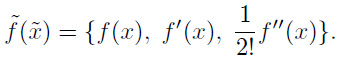
Let f:R→R be an analytic function. Expanding this function in a Taylor Series and evaluating at =x+ϵ (note that we have taken the dual part to be 1) we get
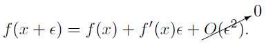 (1)
(1)As we can see, f (x) + f′(x)ϵ is a dual number, so we associate the dual function
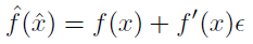 (2)
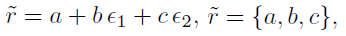
(2)to it. As in the case of the complex numbers, there is an isomorphism between the dual numbers and R2, thus a dual number can be written as
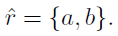 (3)
(3)From now on we will use the notation given by Eq. (3), thus Eq. (2) will be written as
 (4)
(4)The next step is to dualize the composition of f (x) with another function g(x). From the chain rule, we get
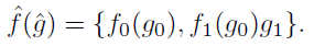 (5)
(5)For instance, if h(x) = f (g(u(x))), the dual component of will be h′(x). That is the power of the dual method of obtaining derivatives. We only need to implement the chain rule once. This makes the dual number method of obtaining derivatives an AD method (forward mode of AD).
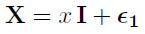
The generalization to second derivatives is straight- forward. To this end we define a new dual number
 (6)
(6)with a, b and c being real numbers and ϵ1 and ϵ2 having the following multiplication table
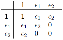 (7)
(7)Now, evaluating the Taylor expansion for f (x) in = x + ϵ1 we have,
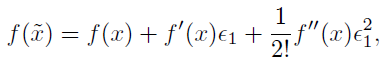 (8)
(8)
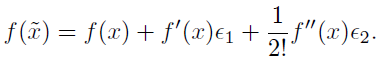 (9)
(9)These expressions are of the form of Eq. (6) so we can write
 (10)
(10)The fact that the third component is a half of the second derivative does not matter. We can choose:
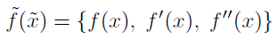 (11)
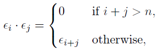
(11)as our definition for this new dual function (in fact, by choosing ϵ2 = 2ϵ2 the factor 1/2 disappears). Also the inappropriate name, new dual function, can be changed to dual function; leaving to the context of the problem (number of components of f ) if we are talking about a simple dual function or of an extended dual function of 3 components. Clearly Eq. (10) can be generalized to obtain higher order derivatives. For instance, to obtain derivatives until order n, define ϵ0 = 1, ϵ1, ϵ2, . . . , ϵn having the multiplication table
 (12)
(12)It is also interesting to prove Eqs. (8, 9, 10) from a matrix algebra point of view. To this end we define the following matrices having the multiplication table (7),
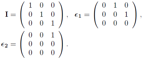 (13)
(13)
 (14)
(14)is in its Jordan canonical form, we will have [32]
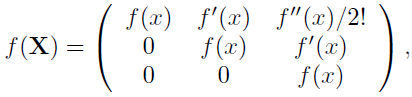 (15)
(15)
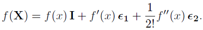 (16)
(16)Thus, the derivatives of f are determined by calculating the matrix function f(X). This matrix function can be calculated by using the Cauchy integral formula for operator-value functions (see for example Sec. 16.8 of [33]).
A generalization of Eqs. (15, 16) to obtain higher order derivatives, can be done by calculating f(X) with
 (17)
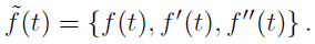
(17)From Eq. (10), the analog of ={x, 1} will be = {x, 1, 0} and the analog of Eq. (4) will be
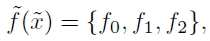 (18)
(18)where f0 = f (x), f1 = f′(x) and f2 = f′′(x). Similarly, we will have
 (19)
(19)for the composition of two dual functions.
Eq. (19), is of central importance in dualizing a function or algorithm. Notice that, unlike the fnite diference methods, the use of Eq. (19) to obtain derivatives does not have the problems of truncation or cancellation errors.
In order to facilitate the use of the dual number given by Eq. (6), it is convenient to introduce a class for this kind of number. In the Matlab programming language, this can be done as:
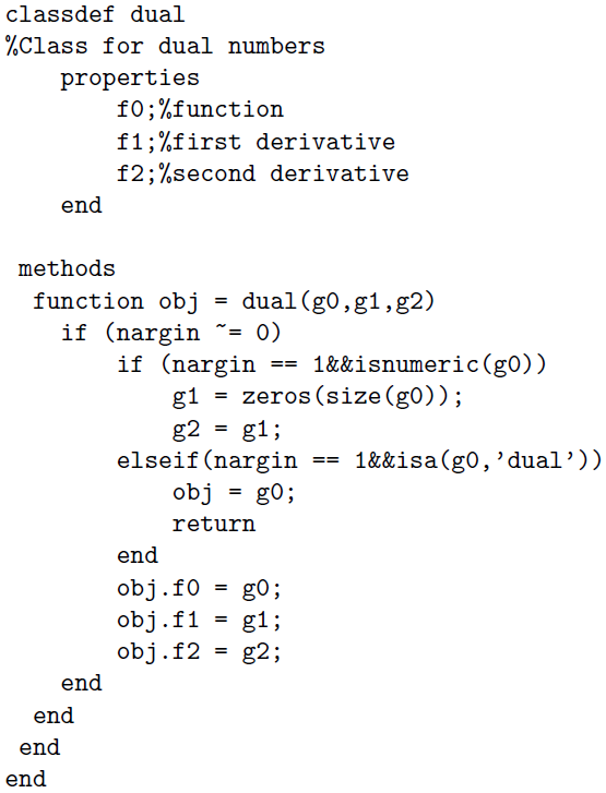
Now, the dual number of Eq. (6) can be written as = dual(a,b,c). This class as well as many other overloaded functions are included in the additional material to this article.
Let us suppose that we are given equation
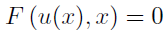 (20)
(20)and that u′(x0) is required. In the case when a closed form expression for u(x) can be obtained, the derivatives can be calculated by writing u(x) in its dual form .
If there is no closed form expression for u(x), applying the chain rule yields
 (21)
(21)Assuming that there are closed form expressions for ∂F/∂x and ∂F/∂u, the derivative u′(x0) can be calculated by solving numerically Eq. (20) and substituting u(x0) into Eq. (21). If ∂F/∂x and ∂F/∂u cannot be obtained in closed form, its numerical values can be obtained using AD. Nevertheless, by coding the dual version of some numerical solution method to solve Eq. (20), we will obtain u(x0) and automatically its derivatives. In the present paper, we dualize the Newton– Raphson method [34, 35].
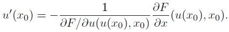
Let f (q) be a real function of a real variable. The Newton–Raphson method allows finding a solution of the equation f (q) = 0. Starting to look for a solution in q0, the algorithm determines an approximate solution as2
 (22)
(22)In order to obtain u′(x0) from Eq. (20) we proceed as follows: Write for the dual version of the function F . Define the dual starting point = {u0, 0, 0}. Since we need F′(u), we define = {x0, 0, 0} and = {u0, 1, 0}, then from 1 = we obtain the first and second derivatives of F with respect to u. This is an extra bonus of the method: we do not need to worry about the derivative of F. In practice, this is an issue, and the derivative must be provided by hand. Finally, write Eq. (22) in its dual form, keeping in mind that since we want u′(x) we need to evaluate in and = {x0, 1, 0}.
Putting = u0d, = x0d, and = fd; the essential part of the method is
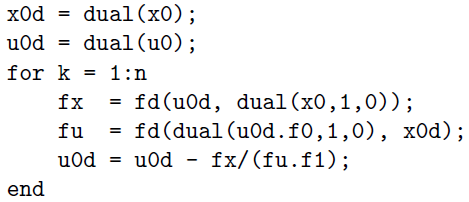
This algorithm will produce. Using Eq. (19), we can construct the general dual function for u:. The complete algorithm is coded in the function NR -dual of the additional material. We also coded Halley’s method [37], so the user can choose between the simple Newton–Raphson method or Halley’s method. Some examples are presented in Section 3.
Let P: A ⊂ R → B ⊂ R be the function representing a cubic spline interpolation and let f b a real function such that f (P (x), x) is defined. The problem is to find f′(P (x), x) with x A. We solve this problem by writing the dual version of the natural cubic spline interpolation.
Suppose that we have n data points (x1, y1), . . . , (xn, yn) , n > 1. A cubic spline is a spline constructed of piecewise third-order polynomials which oass thtough this set of points.
 (23)
(23)In determining the coefficient of the ith piece of the spline, a linear system of 4(n-1)-2 equations and 4(n-1) unknowns will appear [38]. Two more equation can be obtained by demanding that Y ′′(0) = 0 and Y ′′(1) = 0. This yields the so called natural cubic spline interpolation. With this, the coefficients of Yi are given by
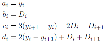 (24)
(24)where the Ds numbers are determined by solving the symmetric tridiagonal system:
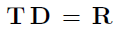 (25)
(25)with
 (26)
(26)
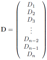 (27)
(27)
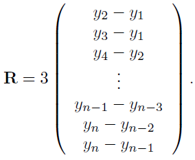 (28)
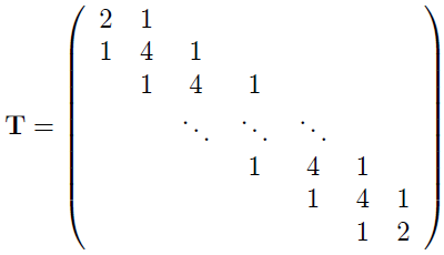
(28)The inversion of an n x n tridiagonal matrix can be done by an O(n) algorithm [34], and in general it is this kind of algorithm which is used in order to find the inverse of the matrix T in Eq. (26). However, as we will show, an analytical formula for the inverse of T can be obtained.
Let us consider the n x n nonsingular tridiagonal matrix
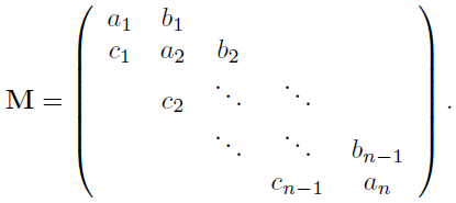
The inverse of such a matrix can be written as [39]:
 (29)
(29)where θi is obtained by solving the recurrence equation
 (30)
(30)with θ0 = 1 and θ1 = a1. Then φi is obtained by solving the recurrence equation
 (31)
(31)The use of Eq. (29) is not an eficient way to find the inverse of a tridiagonal matrix. However it can be used to deduce an analytical formula for the inverse of the matrix T.
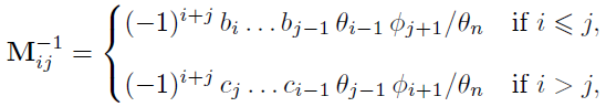
Applying Eqs. (29, 30 and 31) to Eq. (26), we get
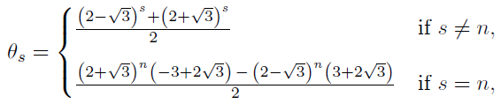 (32)
(32)
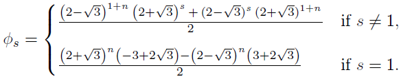 (33)
(33)
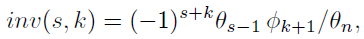 (34)
(34)writing explicitly φk+1/θn and carrying out some elementary algebra, we obtain
 (35)
(35)with
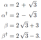 (36)
(36)From this, the inverse of the matrix T is
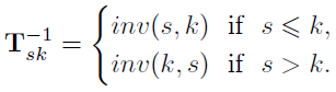 (37)
(37)Thus the coefficients Ds are given by
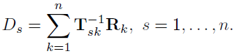 (38)
(38)Now that all the coeficients have been determined, the parametric equation for the interpolated points will be
 (39)
(39)Eliminating the parameter t, the equation for the ith polynomial of the normal cubic spline will be
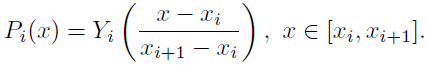 (40)
(40)The interpolated points in the whole interval [x1, xn] are
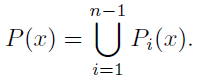 (41)
(41)Once P (x) has been promoted to a dual function (see the function NCSplinedual of the aditional material), the derivatives of an arbitrary function f = f (P (x), x) for any x ∈ [x1, xn],as well as P′(f (x), x), are calculated by writing f in its dual form. Some examples are presented in Section 3.
Let us consider the following ordinary diferential equation (ODE)
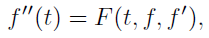 (42)
(42)with initial conditions f (t0) = f0 and f′(t0) = v0. Let g(t) be a function defined in such a way that f (g(t)) and g(f (t)) are defined. The problem we want to address is to find the derivatives of the composition of the functions f and g.
One of the most often used methods for numerically solv- ing ODEs is the Runge–Kutta Method [34,35,40]. In or- der to calculate f′(g(t)), f′′(g(t)), g′(f (t)) and g′′(f (t)), we will dualize the 4th order Runge–Kutta method (RK4). Putting x2 = f′, x1 = f , u1(t, x1, x2) = x2, u2(t, x1, x2) = F (t, x1, x2), the RK4 method produces x2 and x1 and hence f′′(t). From this, the dual ver- sion of f as a function of the real variable t (see the rk4 function of the additional material) is
 (43)
(43)The dual version of f for any dual variable, namely, can be constructed following Eq. (19). (See the rk4dual function of the additional material). Once we have, the derivatives are calculated from the com- positions and—actually, we can calculate the derivatives of any function G(f (t), t). Some exam- ples are presented in Section 3.
All the examples and required folders are included in the additional material to this article.
Suppose that u(x) is defined by the equation f (u, x) = 0 where

Let us consider the functions g1(x) = sin(u(x)) + x and g2(x) = u(sin x + x2). The problem is to find u(x0), u′(x0), u′′(x0), g1(x0), g1′ (x0), g1′′(x0), g2(x0), g2′ (x0), g2′′(x0), with x0 = 0.7. This can be accom- plished by writing the Newton–Raphson algorithm in its dual form. Such an algorithm is coded in the function NR_dual(NRkind,u0,n,fd,gdual). In this function, NRkind is the kind of method used. NRkind = NR1 is for the simple Newton–Raphson method and NRkind = NR2 is for Halley’s method, u0 is the dual point where the method starts to look for a solution, n is the number of iterations, fd is the equation to solve; in this example it will be, the dual version of f (u, x); gdual is the dual point where we want to evaluate the functions. The following script computes the required values.
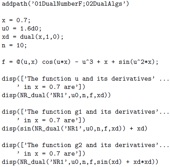
Notice the advantages of this method: we can calculate very complicated derivatives involving u(x) by using the dual functions. The results are shown in Table 1.
Results for the Newton-Raphson example 1

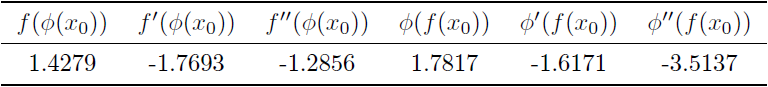
The example here presented concerns the RRRCR spa- tial mechanism [28]. Following Eq. (2) of [28] and the definitions given in the aforementioned reference, the output angle as a function of the input angle is given by the equation
 (44)
(44)Now, if one is interested in calculating the velocities and accelerations, complicated functions involving φ and φ′(θ) will appear. As an example, let us consider the function f (x) = 2 sin2 x and the point x0 = 2.0. The problem is to calculate f (φ(x0)), f′(φ(x0)), f′′(φ(x0)), φ(f (x0)), φ′(f (x0)) and φ′′(f (x0)) for the same set of parameters given in [28], and reproduced in Table 2 for clarity.
Parameters used for the Newton{Raphson example 2
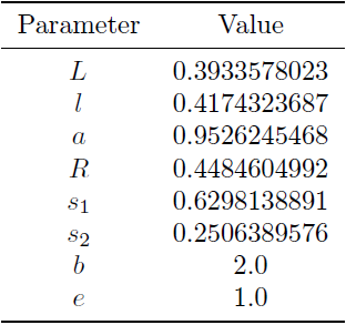
Analogously to the example in Section 3.1, we obtain the results shown in Table 3. Notice that the solution of Eq. (44) for θ = 2 is not unique. The values in Table 3 are for φ = 2.1351.
Results for the Newton{Raphson example 2.
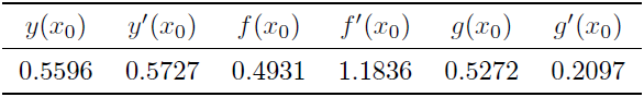
Let y(x) be the normal cubic spline interpolation for the data shown in Table 4.
Points used for the dual cubic spline interpolation example 1.
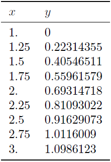
The values y(x0), y′(x0), f (x0), f′(x0), g(x0) and g′(x0) with f (x) = x sin2(y(x)), g(x) = y(x sin2 x) and x0 = 1.75 can be calculated by dualizing the normal cubic spline interpolation method. This has been done in the function NCSplinedual (A,xd). In such a function, A is the matrix containing the points for which the spline will be constructed (in this case, they would be the points of Table 4) and xd is the dual point where we want to evaluate, in this case xd=dual (1.75,1,0). For instance the first (sec- ond) component of NCSplinedual(A,xd) will be y(x0) (y′(x0)).
The derivatives f′(x0) and g′(x0), respectively, are obtained by taking component f1 of

and

The results are given in Table 5.
Results for the dual cubic spline interpolation example 1
This example concerns the determination of the thermal properties of a solid using photothermal radiometry [24]. In particular, we are interested in determining the thermal di_usivity from the experimental data of table. 4 from [24]. The experimental data can be extracted using EasyNData [41]. Assuming that such data are stored in the matrix pts, the dual cubic spline interpolation is done by NCSplinedual (pts,x). Now, according to [24], the thermal diffusivity can be calculated from
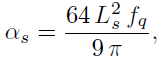 (45)
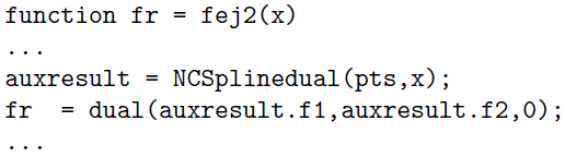
(45)where Ls = 522 µm is the thickness of the studied sample and fq is the frequency for which the derivative of the amplitude of the radiometry signal is zero. The frequency fq can be calculated using the Newton–Raphson algorithm. To this end we define the dual function fej2(x) containing the first and second derivatives of the spline. The essential part of the code is
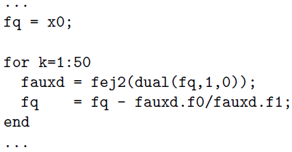
Taking x0 = 10.0 as the initial point where the Newton–Raphson algorithm will start to look for a solution, fq can be found by
After this, the obtained thermal diffusivity was αs =6.00 10−6 m 2s−1 which is in good agreement with the value reported in [24, 42].
Consider the Du_ng equation studied in [27]
 (46)
(46)with initial conditions
 (47)
(47)The values f (t), (f g)(t), (g f )(t), as well as their first and second derivatives at t = 1.0 (or at some other t where the functions are defined) for the function g(t) = sin t (or some other function where the above compo- sitions are defined) can be calculated by dualizing the Runge–Kutta algorithm. Such an algorithm is dualized in the function rk4dual(u1,u2,t0,x10,x20,np,td). In this function, x10 and x20 are the initial conditions for f (t0) and f′(t0) respectively (see Section 2.3.3 for details and also for the definitions of u1 and u2); td is the dual point where we want to evaluate the solution; and np is the number of steps between t0 and and the real component of td. The values for f (t), (f g)(t), (g f )(t), as well as their first and second derivatives at t = 1.0 are shown in Table 6.
Results for the Runge-Kutta example. The functions are evaluated at t = 1:0.

After a dualization of the normal cubic spline interpo- lation algorithm, the Runge–Kutta algorithm, and the Newton–Raphson algorithm, it is possible to calculate the derivatives of functions efficiently, precisely, and accurately. So we can calculate the derivatives of functions depending on the solution of algebraic or differential equations as well as functions resulting from the spline interpolation of experimental data. As an added value to the normal cubic spline interpolation algorithm, it is shown that a closed form expression for its coefficients can be obtained. Interesting applications in science and engineering were studied. Those examples can be used as a guide to dualize many other functions and algorithms. For example, it would be interesting to dualize the trapezium rule although this would be only for aca- demic purposes since there is not much to gain because its components would be the integral, the first derivative (which is actually the function to integrate), and the second derivative (which is actually the first derivative of the function to integrate). Nevertheless, the dualization of an integration method could be necessary for dualizing some other algorithm.
Results for the Newton-Raphson example 1
Parameters used for the Newton{Raphson example 2
Results for the Newton{Raphson example 2.
Points used for the dual cubic spline interpolation example 1.
Results for the dual cubic spline interpolation example 1
Results for the Runge-Kutta example. The functions are evaluated at t = 1:0.
