Optimal tracking in two-degree-of-freedom control systems: Coupled
					tank system

P. Teppa-Garran; M. Faggioni; G. Garcia

Articles

Received: 07 June 2022

Accepted: 26 January 2023

Published: 31 August 2023

DOI: https://doi.org/10.22201/icat.24486736e.2023.21.4.2000

Funding

Funding source: Research Program of the Metropolitan University in Caracas, Venezuela

Contract number: PG-A-14-21-22

Abstract: This article presents an optimal design of a two-degree-of-freedom (2-DoF) controller that will lead to zero asymptotic steady-state tracking error. The reference inputs are chosen from the set of steps, ramps, and other persistent signals used currently. The main idea is to transform the tracking 2-DoF problem into an equivalent state-space feedback-control synthesis one. Where, an internal model of the reference input is introduced. Then, through the linear quadratic regulator (LQR) technique, the desired performance objectives are addressed by minimizing a quadratic cost function. Finally, the computed state-feedback optimal gains are linked to the polynomials used within the 2-DoF formalism. The fundamental aspect of the design is that it only utilizes the measurable information of the plant provided by its inputs and outputs and takes advantage of efficient state-space numerical algorithms. The proposed method is applied to a coupled-tank system, the results achieved confirm the effectiveness of the approach.

Keywords: Tracking problem, reference following, two-degree-of-freedom controller, 2 DoF, LQR, coupled-tank system.

1. Introduction

Two fundamental problems arise in the design of control systems. Reference tracking and disturbance attenuation. It is widely known that both problems are produced by the corresponding closed-loop transfer functions (sensitivity and complementary sensitivity) (Safonov et al., 1981). While disturbance attenuation is exclusively a feedback problem, the tracking problem, which is associated with an open-loop property, can be solved by using a suitable precompensator. Therefore, the tracking problem is conveniently managed within the two-degree-of-freedom (2-DoF) control configuration. In a classical feedback control scheme, the control signal is obtained through the difference between the reference and the current output. Since there is only one input to the controller, this classical control structure is also called a one-degree-of-freedom (1-DoF) controller. Although 1-DoF controllers have many nice structural properties (Davison, 1976), a compromise must be reached to solve simultaneously the tracking and disturbance attenuation problems. On the other hand, a controller has 2-DoF, when the reference signal and the plant output can be processed independently to obtain the control signal. The advantages of using a 2-DoF control system are well known: the closed-loop properties can be configured independently of the reference tracking transfer function (Grimble, 1994). This possibility results from the separation between the response to the reference signal and the feedback transfer function.

Among the first contributions of the 2-DoF theory, it is worth mentioning (Horowitz, 1963; Vidyasagar, 1985). Since then, it can be found many published research results on the design of 2-DoF controllers. Hoyle et al. (1991) and Limebeer et al. (1993) developed a 2-DoF extension of the $H_{\infty}$ loop-shaping design method created by McFarlane and Glover (1992) to enhance the model-matching properties of the closed-loop. Shaked and De Souza (1995) worked in a game theory $H_{\infty}$ strategy to solve the tracking problem of a known in advance (non-causal) or measured online (causal) reference signal. Prempain and Bergeon (1998) utilized Youla parametrization and defined a design method consisting in two steps. In the first step of the procedure, a model-matching approach is used to set the desired nominal tracking objectives, while a μ-synthesis technique is implemented to achieve the robust performance objectives in the second step. Kim and Tsao (2002) address the tracking of near-periodic-time-varying signals to propose a unified method to design simultaneously previewed feedforward, feedback, and repetitive control. Liu et al. (2007) developed a 2-DoF control scheme for decoupling multiple-input-multiple-output processes in the presence of time delays. Hanif (2013) consider an active damping technique by introducing a 2-DoF PID control structure in grid connected photovoltaic systems. Mateo and Sugimoto (2015) formulated a method to tune a prefilter and the feedforward controller of the 2-DoF configuration. Vargas et al. (2016) present a practical design of longitudinal stability and control augmentation system (SCAS) using a 2-DoF control scheme. Zhang and Xia (2017) used a 2-DoF control approach for non-minimum phase systems with time delay. Ahmad (2018) achieves precise reference tracking performance from a piezoelectric positioning stage proposing a 2-DoF robust digital controller. Zaky et al. (2018) present a 2-DoF and variable structure control schemes for induction motor drives. Teppa-Garrán and Vásquez (2020) utilize a feedforward anticipation control of a desired reference signal whose temporal derivatives are known to conduct the control of a rotary flexible joint. Finally, Vavilala and Thirumavalavan (2021) consider the tuning of the 2-DoF FOIMC based on the Smith predictor.

The problem of optimization of the 2-DoF structure has not received wide attention. Nevertheless, some interesting works can be mentioned. The initial contributions of Limebeer et al. (1993) and Grimble (1994), where the problem is formulated into a general framework. The approach of Hoover et al. (2004) which propose a simple single-input-single-output 2-DoF pole-placement design method that provides $l_{2}$ -optimal tracking of a given reference signal and Vilanova (2008), where the problem of optimal design of the reference controller have been addressed by the optimization of a linear quadratic Gaussian type cost function. Always within the framework of 2-DoF formulation, some applications using advanced optimization algorithms have been treated, but in the context of PID controller synthesis (Kim, 2002; 2004; Sigiura, 1996; Zhan et al., 2002).

This paper deals with the problem of optimal design of a 2-DoF controller that will lead to zero asymptotic steady-state tracking error. The reference inputs can include steps, ramps, and other persistent signals used currently. The main idea is to translate the tracking 2-DoF problem into a state-space- feedback control synthesis one (Garcia, Tarbouriech & Turner, 2011). Where, an internal model of the reference input is introduced (Francis & Wonham, 1976). Then, through the LQR method the desired performance objectives are addressed by minimizing a quadratic cost function (Anderson & Moore, 2007; Lewis & Syrmos, 1995). Finally, the state-feedback optimal gains are linked to the polynomials used within the 2-DoF formalism. A fundamental aspect of the method is that it only utilizes the measurable information of the plant provided by its inputs and outputs.

The article is organized as follows. Section 2 considers the problem formulation. Section 3 provides the main result of the work, where it is stablished a connection between the 2-DoF system and the state-feedback control synthesis problem. Finally, Section 4 shows the effectiveness of the method by considering its application to a coupled-tank system.

Notation: Capital bold typeface letters denote matrices and small bold typeface letters denote vectors. $\dot{a} = d a / d t, \ddot{a} (t) = d^{2} a / d t^{2}, a^{(i)} (t) = d^{i} a / d t^{i}$ , $R$ is the set of real numbers and $A^{T} = t r a n s p o s e o f A$ .

2. Problem formulation

Consider a plant described by

D (p) y (t) = N (p) u (t)

(1)

where $y (t) \in R$ is the plant output and $u (t) \in R$ the plant input. $N (p)$ and $D (p)$ are polynomials and $p$ is equal to the time differential operator $d / d t$ or the Laplace complex variable $s$ . Polynomials $D (p)$ and $N (p)$ are defined by

D (p) = p^{n} + \sum_{i = 0}^{n - 1} a_{i} p^{i}, N (p) = \sum_{i = 0}^{m} b_{i} p^{i}

(2)

with $a_{i} \in R$ and $b_{j} \in R$ for all $i = 0, \dots, n - 1$ and $j = 0, \dots, m$ . The order of the system is defined as the degree of $D (p)$ . We also suppose that the system is controllable. In this case, polynomials $D (p)$ and $N (p)$ , must be coprime (Antsaklis & Michel, 2006).

A general 2-DoF controller (Landeau & Gianluca, 2006) can be described by

L (s) u (s) = T (s) y_{r} (s) - R (s) y (s)

(3)

where $y_{r} (t) \in R$ is the input reference and the polynomials $L (s), T (s)$ and $R (s)$ are written as

\begin{matrix} L (s) = \sum_{i = 0}^{n_{L}} l_{i} s^{i} \\ T (s) = \sum_{i = 0}^{n_{T}} t_{i} s^{i} \\ R (s) = \sum_{i = 0}^{n_{R}} r_{i} s^{i} \end{matrix}

(4)

the controller can be thought as a combination of a feedback having the transfer function $G_{f b} (s) = R (s) / L (s)$ and a feedforward with transfer function $G_{f f} (s) = T (s) / L (s)$ .

A block diagram of the control system is shown in Fig. 1 and an implementation of the controller that highlights the polynomials in (4) is included in Fig. 2.

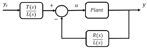
Figure 1
General 2-DoF control system structure.

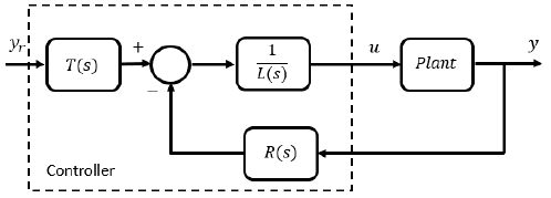
Figure 2
Polynomials in 2-DoF control system.

The general problem under study can be formulated as follows:

Problem 1: Given the plant (1), find polynomials $L (s), T (s)$ and $R (s)$ in (3) to compute the control input $u (t)$ so that the controlled output $y (t)$ tracks asymptotically a predefined reference input $y_{r} (t)$ in the 2-DoF control system of Fig. 2.

In the next section, the preceding tracking problem will be solved within a state-space formulation using an optimal LQR approach.

3. Proposed method

In this section, we consider the problem of designing a 2-DoF controller that provides asymptotic tracking of a predefined reference input with zero steady-state error. The reference inputs include steps, ramps and other persistent signals currently used. The main idea is to translate the tracking 2-DoF problem into a state-space- feedback control synthesis one.

3.1. Plant and state-space model connection

Using the input - output information of the plant, it is defined the state vector

x (t) = [\begin{matrix} y (t) \\ ⋮ \\ y^{(n - 1)} (t) \\ u (t) \\ ⋮ \\ u^{(n_{u} - 1)} (t) \end{matrix}] \in R^{N} (N = n + n_{u})

Associated with system (1), we define the following state-space system model:

\begin{matrix} \dot{x} (t) = A x (t) + B u^{(n_{u})} (t) \\ = [\begin{matrix} A_{11} & A_{12} \\ 0 & A_{22} \end{matrix}] x (t) + [\begin{matrix} 0 \\ 1 \end{matrix}] u^{(n_{u})} (t), n_{u} \geq m \\ y (t) = C x (t) = [\begin{matrix} 1 & 0 \end{matrix}] x (t) \end{matrix}

(5)

the partitioned matrices $A_{11}, A_{12}$ and $A_{22}$ are defined as

A_{11} = [\begin{matrix} 0 & 1 & 0 & 0 & \dots & 0 \\ 0 & 0 & 1 & 0 & \dots & 0 \\ ⋮ & ⋮ & ⋮ & ⋮ & ⋱ & ⋮ \\ 0 & 0 & 0 & 0 & \dots & 1 \\ - a_{0} & {- a}_{1} & {- a}_{2} & {- a}_{3} & \dots & {- a}_{n - 1} \end{matrix}]

A_{12} = [\begin{matrix} 0 & \dots & 0 & 0 & \dots & 0 \\ 0 & \dots & 0 & 0 & \dots & 0 \\ ⋮ & \dots & ⋮ & ⋮ & \dots & ⋮ \\ 0 & \dots & 0 & 0 & \dots & 0 \\ b_{0} & \dots & b_{m} & 0 & \dots & 0 \end{matrix}]

A_{22} = [\begin{matrix} 0 & 1 & 0 & \dots & 0 \\ 0 & 0 & 1 & \dots & 0 \\ ⋮ & ⋮ & ⋮ & ⋱ & ⋮ \\ 0 & 0 & 0 & \dots & 1 \\ 0 & 0 & 0 & \dots & 0 \end{matrix}]

see the appendix for an example of the connection between Equations (1) and (5). The only condition on $n_{u}$ is $n_{u} \geq m$ . From a practical point of view, some care must be taken to obtain proper and then realizable compensators. One condition which ensures that proper compensator will be obtained is $n_{c} \geq n - 1$ which corresponds to the minimal order observer in the case of a single output system (Antsaklis & Michel, 2006).

3.2. Controllability

For this work, it is important to assure the controllability of the equivalent state-space model.

Theorem 1: If System (1) is controllable, then System (5) is controllable, if and only if all the roots of polynomial $N (s)$ in (2) are different of zero.

Proof: A step-by-step procedure shows that the transfer function of System (5) gives $G (s) = N (s) / s^{n_{u}} D (s) .$ If System (1) is controllable, polynomials $N (s)$ and $D (s)$ are coprime. Then, if all the roots of $N (s)$ are different of zero, it follows that $N (s)$ and $s^{n_{u}} D (s)$ are coprime implying the controllability of System (5) and completing the proof.

3.3. Optimal tracking of a step reference

A fundamental result of the control theory is that zero-state tracking errors are achieved by considering in the control policy a suitable model of the dynamic structure of the reference signal (Francis & Wonham, 1976). Let the tracking error $e (t)$ be equal to

e (t) = y_{r} (t) - y (t)

(6)

taking the derivative of (6) and using the output equation of the state-space Model (5) yields

\dot{e} (t) = 0 - \dot{y} (t) = - C \dot{x} (t)

(7)

now, taking the derivative of the state Equation (5) gives

\ddot{x} (t) = A \dot{x} (t) + B u^{(n_{u} + 1)} (t)

(8)

Equations (7) and (8) can be combined as

\dot{z} (t) = A_{a} z (t) + B_{a} u_{0} (t)

(9)

where the augmented state vector is $z (t) = {[\begin{matrix} e (t) & \dot{x} (t) \end{matrix}]}^{T}$ and the input is taken as $u_{0} (t) = u^{(n_{u} + 1)} (t)$ which results in the following matrices $A_{a}$ and $B_{a}$

A_{a} = [\begin{matrix} 0 & - C \\ 0 & A \end{matrix}], B_{a} = [\begin{matrix} 0 \\ B \end{matrix}]

to have a LQR formulation of the tracking problem, the following quadratic cost is considered

J = \int_{0}^{\infty} [{z (t)}^{T} Q z (t) + ρ {u_{0} (t)}^{2}] d t

(10)

where $Q$ is a positive semi-definite matrix which has an impact on the closed-loop transient response and parameter $ρ > 0$ can be used to tune the amplitude of the control signal. It is well known (Anderson & Moore, 2007; Lewis & Syrmos, 1995) that the state feedback control

u_{0} (t) = - K z (t)

(11)

minimizes (10) and stabilizes System (9) with the vector $K$ equal to

K = - ρ^{- 1} {B_{a}}^{T} P

(12)

here $P$ is the symmetric positive definite solution of the continuous algebraic Riccati equation given by

{A_{a}}^{T} P + P A_{a} - ρ^{- 1} P B_{a} {B_{a}}^{T} P + Q = 0

(13)

since, it can be easily verified that the System (9) with matrices $A, B$ and $C$ from (5) is controllable. We can find constant $K_{1}$ and vector gain $K_{2}$ in (11) (here vector $K$ has been partitioned according to the dimensions of the components of vector $z$ ) such that the system (9) is stable, and the quadratic cost (10) is minimized. After performing time-integration in (11), the control signal $u^{(n_{u})} (t)$ in (5) yields

u^{(n_{u})} (t) = {- K}_{1} \int_{0}^{t} e (τ) d τ - K_{2} x (t)

(14)

next, Equation (14) is developed to find the relation between the gains $K_{1}$ and $K_{2}$ with the polynomials $L (s), T (s)$ and $R (s)$ in (3). Using the state-vector $x (t)$ from (5) gives

u^{(n_{u})} (t) = {- K}_{1} \int_{0}^{t} e (τ) d τ - K_{2} [\begin{matrix} y (t) \\ ⋮ \\ y^{(n - 1)} (t) \\ u (t) \\ ⋮ \\ u^{(n_{u} - 1)} (t) \end{matrix}]

the vector gain $K_{2}$ is partitioned as $[\begin{matrix} K_{2 y} & K_{2 u} \end{matrix}]$

u^{(n_{u})} = {- K}_{1} \int_{0}^{t} e (τ) d τ - [\underset{K_{2 y}}{\underset{⏟}{\begin{matrix} r_{0} & \dots & r_{n - 1} \end{matrix}}}] [\begin{matrix} y (t) \\ ⋮ \\ y^{(n - 1)} (t) \end{matrix}]

- [\underset{K_{2 u}}{\underset{⏟}{\begin{matrix} l_{0} & \dots & l_{n_{u} - 1} \end{matrix}}}] [\begin{matrix} u (t) \\ ⋮ \\ u^{(n_{u} - 1)} (t) \end{matrix}]

taking the Laplace transform of the above equation yields the 2-DoF controller defined in (3), where the polynomials $L (s), T (s)$ and $R (s)$ can be identified as

L (s) = l_{0} + l_{1} s + \dots + l_{n_{u} - 1} + s^{n_{u}}

T (s) = - K_{1} / s

(15)

R (s) = - K_{1} / s + r_{0} + r_{1} s + \dots + r_{n - 1} s^{n - 1}

these results are summarized in the following theorem.

Theorem 2: Given the Plant (1), the control signal $u (t)$ in (3) for the 2-DoF control system of Fig. 2 can be computed through the polynomials (15) to provide asymptotic tracking for any step reference input $y_{r} (t)$ and minimization of the quadratic cost (10).

3.4. Optimal tracking of a ramp reference

It is easy to show that for a ramp reference input $y_{r} (t),$ the augmented state vector in (9) takes the form

z (t) = {[\begin{matrix} e (t) & \dot{e} (t) & \ddot{x} (t) \end{matrix}]}^{T}

and the control signal is $u_{0} (t) = u^{(n_{u} + 2)} (t)$ . Resulting the matrices $A_{a}$ and $B_{a}$

A_{a} = [\begin{matrix} 0 & 1 & 0 \\ 0 & 0 & - C \\ 0 & 0 & A \end{matrix}], B_{a} = [\begin{matrix} 0 \\ 0 \\ B \end{matrix}]

after taking the integration two times in the control signal $u_{0} (t)$ yields

u^{(n_{u})} (t) = - K_{1} \iint_{0}^{t} e (τ) d t - K_{2} \int_{0}^{t} e (τ) d t - K_{3} x (t)

(16)

the gain vector $K_{3}$ is partitioned as $[\begin{matrix} K_{3 y} & K_{3 u} \end{matrix}]$ to obtain

\begin{matrix} u^{(n_{u})} (t) = - K_{1} \iint_{0}^{t} e (τ) d t - K_{2} \int_{0}^{t} e (τ) d t \\ - [\underset{K_{3 y}}{\underset{⏟}{\begin{matrix} r_{0} & \dots & r_{n - 1} \end{matrix}}}] [\begin{matrix} y (t) \\ ⋮ \\ y^{(n - 1)} (t) \end{matrix}] \\ - [\underset{K_{3 u}}{\underset{⏟}{\begin{matrix} l_{0} & \dots & l_{n_{u} - 1} \end{matrix}}}] [\begin{matrix} u (t) \\ ⋮ \\ u^{(n_{u} - 1)} (t) \end{matrix}] \end{matrix}

after applying the Laplace transform to the above equation, the polynomials $L (s), T (s)$ and $R (s)$ of the 2-DoF structure of Fig. 2 are identified as

\begin{matrix} L (s) = l_{0} + l_{1} s + \dots + l_{n_{u} - 1} + s^{n_{u}} \\ T (s) = - K_{1} / s^{2} - K_{2} / s \\ R (s) = - K_{1} / s^{2} - K_{2} / s + r_{0} + r_{1} s + \dots + r_{n - 1} s^{n - 1} \end{matrix}

(17)

the internal model principle is easily extended to other reference inputs by following the same general procedure outlined for the step and ramp inputs.

4. Results

In this section, the proposed method is applied to a coupled-tank system.

4.1. Coupled tank system

The coupled tank system is given in Fig. 3. The setup experiment also includes a 1.3 MHz Intel Pentium 4 computer and interface to LabVIEW via the data acquisition card of national instrument DAQ-USB-6008. It consists of 8 inputs and 2 analog outputs and 12 digital input/output ports. The sampling period was set to a value of 50 ms. The apparatus is used in the control laboratory at the Simón Bolívar University in Venezuela. It comprises a single pump with two tanks. Each tank is instrumented with a pressure sensor to measure the water level. The pump drives the water from the bottom basin up to the top of the system. Depending on how the outflow valves are configured, the water then flows to the top tank, bottom tank, or both. One configuration is shown in Fig. 4, where the output of the pump is connected to the first tank. The nonlinear state space model (Apkarian, 2013; Grygiel, 2016) is given in (18), here the state vector is equal to the tank’s levels, the control signal corresponds to the input voltage applied to the pump and the output is selected as the second tank level.

\dot{x} (t) = [\begin{matrix} \frac{- C_{1}}{A_{1}} \sqrt{x_{1} (t)} & 0 \\ \frac{C_{1}}{A_{2}} \sqrt{x_{1} (t)} & \frac{- C_{2}}{A_{2}} \sqrt{x_{2} (t)} \end{matrix}] x (t)

+ [\begin{matrix} K_{p} / A_{1} \\ 0 \end{matrix}] u (t)

(18)

y (t) = [\begin{matrix} 0 & 1 \end{matrix}] x (t)

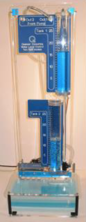
Figure 3
Coupled tank system.

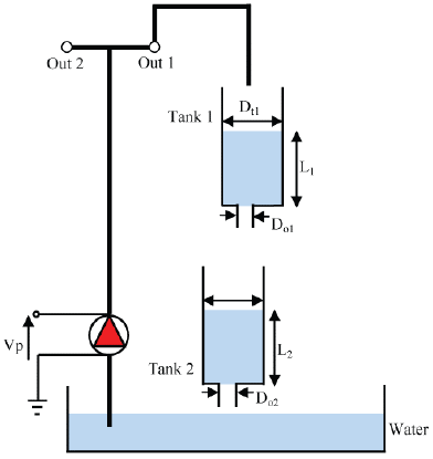
Figure 4
Standard configuration of the coupled tank system.

With $C_{1} = A_{d 1} \sqrt{2 g}, C_{2} = A_{d 2} \sqrt{2 g}, A_{1}$ , and $A_{2}$ denote the cross-sectional area of the tanks 1 and 2, respectively. $A_{d 1}, A_{d 2}$ give the cross-sectional areas of the corresponding orifices, $g$ is the gravitational constant on Earth and $K_{p}$ is the pump flow constant. The nonlinear model is linearizing in the operating point ${[{\tilde{L}}_{1}, {\tilde{L}}_{2}]}^{T}$ resulting in the equations

\begin{matrix} \dot{x} = [\begin{matrix} \frac{- C_{1}}{2 A_{1} \sqrt{{\tilde{L}}_{1}}} & 0 \\ \frac{C_{1}}{2 A_{2} \sqrt{{\tilde{L}}_{1}}} & \frac{- C_{2}}{2 A_{2} \sqrt{{\tilde{L}}_{2}}} \end{matrix}] x + [\begin{matrix} K_{p} / A_{1} \\ 0 \end{matrix}] u \\ y = [\begin{matrix} 0 & 1 \end{matrix}] x \end{matrix}

(19)

the description and numerical values of the physical parameters for the tank system are given in Table 1.

Table 1
Physical parameters of the coupled tank system.

By employing the numerical values from Table 1. It is possible to perform the following calculations

\begin{array}{l} A_{1} = A_{2} = π {(4.445 / 2)}^{2} = 15.53 {c m}^{2} \\ A_{d 1} = π {(0.635 / 2)}^{2} = 0.317 {c m}^{2} \\ A_{d 2} = π {(0.476 / 2)}^{2} = 0.178 {c m}^{2} \\ {\tilde{L}}_{1} = {\tilde{L}}_{2} = 15 c m \end{array}

replacing the previous values in (19) gives the linear model differential equation of the coupled tank system as

\frac{d^{2}}{{d t}^{2}} y (t) + 0.18 \frac{d}{d t} y (t) + 0.008 y (t) = 0.03 u (t)

(20)

4.2. Two-degree-of freedom control system design for tracking a step reference input

Defining the state vector as $x (t) = {[\begin{matrix} y (t) & \dot{y} (t) & u (t) & \dot{u} \end{matrix} (t)]}^{T}$ in (5), the coupled tank system model (20) takes the form

\begin{matrix} \dot{x} = [\begin{matrix} 0 & 1 & 0 & 0 \\ - 0.008 & - 0.18 & 0.03 & 0 \\ 0 & 0 & 0 & 1 \\ 0 & 0 & 0 & 0 \end{matrix}] x + [\begin{matrix} 0 \\ 0 \\ 0 \\ 1 \end{matrix}] \ddot{u} \\ y = [\begin{matrix} 1 & 0 & 0 & 0 \end{matrix}] x \end{matrix}

(21)

here, we have $n = 2$ and it is fixed $n_{u} = 2 .$ For a step reference input, the augmented Model (9) has matrices

A_{a} = [\begin{matrix} 0 & - 1 & 0 & 0 & 0 \\ 0 & 0 & 1 & 0 & 0 \\ 0 & - 0.008 & - 0.18 & 0.03 & 0 \\ 0 & 0 & 0 & 0 & 1 \\ 0 & 0 & 0 & 0 & 0 \end{matrix}]

\begin{matrix} B_{a} = {[\begin{matrix} 0 & 0 & 0 & 0 & 1 \end{matrix}]}^{T} \end{matrix}

using $Q = I_{5}$ and $ρ = 1$ in the quadratic cost (10) produces the gain $K = [\begin{matrix} K_{1} & K_{2} \end{matrix}]$ in (14) as

K = [\begin{matrix} \underset{K_{1}}{\underset{⏟}{- 1}} & \underset{r_{0}}{\underset{⏟}{7.78}} & \underset{r_{1}}{\underset{⏟}{21.57}} & \underset{l_{0}}{\underset{⏟}{1.90}} & \underset{l_{1}}{\underset{⏟}{2.19}} \end{matrix}]

Remark 1: Gain $K$ has been computed using instruction $l q r$ of MATLAB.

From vector $K$ , it is possible to recovery the polynomials $L (s), T (s)$ and $R (s)$ for the 2-DoF control structure. This appears in Fig. 5 for the coupled tank system.

L (s) = l_{0} + l_{1} s + l_{2} s^{2} = 1.90 + 2.19 s + s^{2}

T (s) = - K_{1} / s = 1 / s

R (s) = - K_{1} / s + r_{0} + r_{1} s = 1 / s + 7.78 + 21.57 s

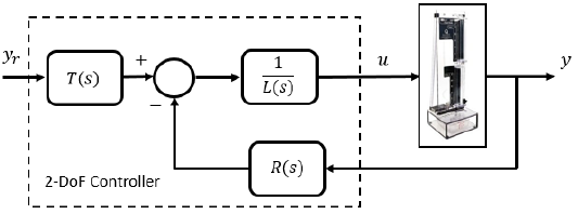
Figure 5
2-DoF control structure for the coupled tank system.

Figure 6 exhibits the tracking ability of the 2-DoF control system structure. Three step changes are considered, and the controller always reacts satisfactorily. Figure 7 shows the pump voltage control signal, which values are always within the voltage technological limits.

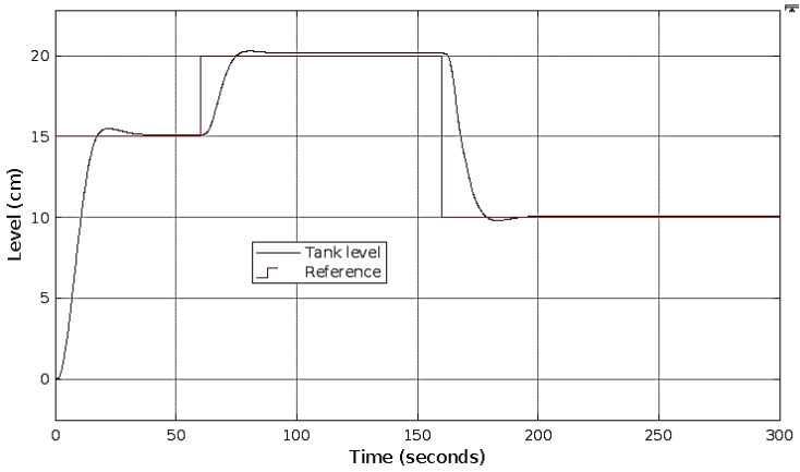
Figure 6
Second tank closed-loop liquid level response of the 2-DoF control system for the tracking problem of a step reference input.

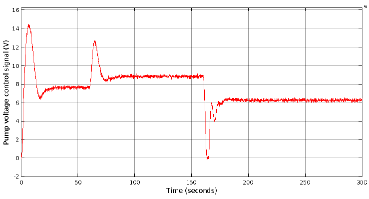
Figure 7
Control signal for step reference input tracking.

4.3. Disturbance rejection

The disturbance attenuation of the design is now studied through the following experiment. The system starts in the standard configuration of Fig. 2, but at $t = 100 s$ switches to that of Fig. 8, where the pump output feeds both Tank 1 and Tank 2. At $t = 200 s,$ it returns to the initial interconnection of Fig. 2. This experiment allows to model a trapezoidal perturbation that operates in the interval $[100; 200] s$ , causing a decrease in the inlet flow to Tank 1 and the appearance of a direct flow in Tank 2.

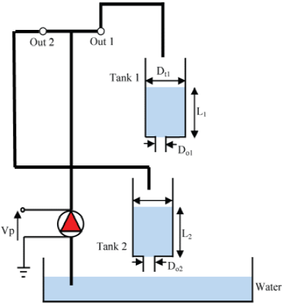
Figure 8
The connection scheme of the coupled tanks system to create a disturbance that decrease the inlet to Tank 1.

Figure 9 allows appreciating the adequate disturbance rejection achieved with the design method. At the instants of time, where the trapezoidal disturbance starts and ends, the 2-DoF controller reacts by returning the controlled output to the reference level. Figure 10 allows watching the control signal evolving within the limits of the tank pump.

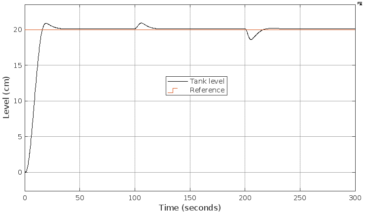
Figure 9
Second tank closed-loop liquid level response for disturbance rejection.

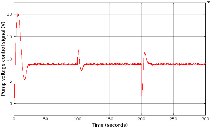
Figure 10
Coupled-tank-system control signal for trapezoidal disturbance rejection.

4.4. Two-degree-of freedom control system design for tracking a ramp reference input

For a ramp reference input, the augmented Model (9) has matrices

A_{a} = [\begin{matrix} 0 & 1 & 0 & 0 & 0 & 0 \\ 0 & 0 & - 1 & 0 & 0 & 0 \\ 0 & 0 & 0 & 1 & 0 & 0 \\ 0 & 0 & - 0.008 & - 0.188 & 0.03 & 0 \\ 0 & 0 & 0 & 0 & 0 & 1 \\ 0 & 0 & 0 & 0 & 0 & 0 \end{matrix}]

(23)

\begin{matrix} B_{a} = {[\begin{matrix} 0 & 0 & 0 & 0 & 0 & 1 \end{matrix}]}^{T} \end{matrix}

using $Q = I_{6}$ and $ρ = 1$ in the quadratic cost (10) produces the gain $K = [\begin{matrix} K_{1} & K_{2} & K_{3} \end{matrix}]$ in (16) as

K = [\begin{matrix} \underset{K_{1}}{\underset{⏟}{- 1}} & \underset{K_{2}}{\underset{⏟}{- 8.05}} & \underset{r_{0}}{\underset{⏟}{31.09}} & \underset{r_{1}}{\underset{⏟}{58.55}} & \underset{l_{0}}{\underset{⏟}{3.02}} & \underset{l_{1}}{\underset{⏟}{2.65}} \end{matrix}]

the polynomials $L (s), T (s)$ and $R (s)$ are identified as

L (s) = l_{0} + l_{1} s + s^{2} = 3.02 + 2.65 s

T (s) = - K_{1} / s^{2} - K_{2} / s = \frac{1}{s^{2}} + \frac{8.05}{s}

\begin{matrix} R (s) = - K_{1} / s^{2} - K_{2} / s + r_{0} + r_{1} s \\ = \frac{1}{s^{2}} + \frac{8.05}{s} + 31.09 + 58.55 s \end{matrix}

The reference input applied to the coupled tank system is shown in Fig. 11, here a combination of ramps with different slopes and step changes are considering. The comparison between the reference input and the controlled output is displayed in Fig. 12, while the evolution of the control signal is found in Fig. 13.

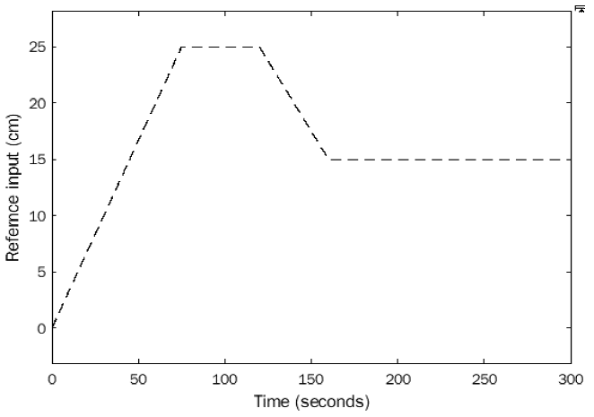
Figure 11
Ramp reference input to validate the 2-DoF controller design.

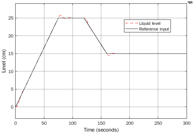
Figure 12
Second tank closed-loop liquid level response for ramp reference tracking.

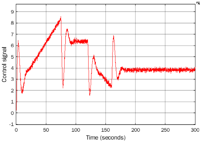
Figure 13
Coupled-tank-system control signal for ramp reference tracking.

Conclusions

In this work, it has been proposed a method to design an optimal 2-DoF control system that provides zero asymptotic steady-state tracking error to a predefined reference input. The reference inputs include steps, ramps, and other persistent signals used currently. The plant is described by an input-output model and then it is translated into an equivalent state-space model which state vector depends exclusively on the measurable information of the original system. It is established that the controllability of the state space model implies the controllability of the original system. This allows using the efficient machinery of state-feedback-controller-synthesis and then, connect the results of the state-space synthesis with the polynomials of the 2-DoF controller. The internal model principle is employed to augment the equivalent state-space model depending on the reference input considered.

Acknowledgements

The authors are grateful for the support provided by the Research Program of the Metropolitan University in Caracas, Venezuela through project number PG-A-14-21-22.

References

Ahmad, I. (2018). Two degree-of-freedom robust digital controller design with Bouc-Wen hysteresis compensator for piezoelectric positioning stage. IEEE Access, 6, 17275-17283. https://doi.org/10.1109/ACCESS.2018.2815924.

Anderson, B. D., & Moore, J. B. (2007). Optimal control: linear quadratic methods. Courier Corporation.

Antsaklis, P. J., & Michel, A. N. (2006). State feedback and state observers. Linear Systems, 321-382. https://doi.org/10.1007/0-8176-4435-0_4.

Apkarian, J., Lacheray, H., & Abdosalami, A. (2013). Instructor Workbook. Coupled Tanks Experiment for Matlab/Simulink Users. Quanser Innovate Educate.

Davison, E. (1976). The robust control of a servomechanism problem for linear time-invariant multivariable systems. IEEE transactions on Automatic Control, 21(1), 25-34. https://doi.org/10.1109/TAC.1976.1101137.

Francis, B. A., & Wonham, W. M. (1976). The internal model principle of control theory. Automatica, 12(5), 457-465. https://doi.org/10.1016/0005-1098(76)90006-6.

Garcia, G., Tarbouriech, S. & Turner, M. (2011). Output feedback control design for linear systems subject to amplitude and dynamics saturating actuators and sensors. LAAS Internal Research Report.

Grimble, M. J. (1994). Robust industrial control: Optimal design approach for polynomial systems. New Jersey, USA, Prentice-Hall International.

Grygiel, R., Bieda, R., & Blachuta, M. (2016). On significance of second-order dynamics for coupled tanks systems. In 2016 21st International Conference on Methods and Models in Automation and Robotics (MMAR) (pp. 1016-1021). IEEE. https://doi.org/10.1109/MMAR.2016.7575277.

Hanif, M., Khadkikar, V., Xiao, W., & Kirtley, J. L. (2013). Two degrees of freedom active damping technique for LCL filter-based grid connected PV systems. IEEE Transactions on Industrial Electronics, 61(6), 2795-2803. https://doi.org/10.1109/TIE.2013.2274416.

Hoover, D. N., Longchamp, R., & Rosenthal, J. (2004). Two-degree-of-freedom ℓ2-optimal tracking with preview. Automatica, 40(1), 155-162. https://doi.org/10.1016/j.automatica.2003.09.003.

Horowitz, I. M. (1963). Title of chapter in the book, Synthesis of feedback systems, ist ed.

Hoyle, D. J., Hyde, R. A., & Limebeer, D. J. (1991). An h/sub infinity/approach to two degree of freedom design. In [1991] Proceedings of the 30th IEEE Conference on Decision and Control (pp. 1581-1585). IEEE. https://doi.org/10.1109/CDC.1991.261671.

Kim, B. S., & Tsao, T. C. (2002). An integrated feedforward robust repetitive control design for tracking near periodic time varying signals. Japan-USA on Flexible Automation, Japan.

Kim, D. H. (2002). Tuning of 2-DOF PID controller by immune algorithm. In Proceedings of the 2002 Congress on Evolutionary Computation. CEC'02 (Cat. No. 02TH8600) (Vol. 1, pp. 675-680). IEEE. https://doi.org/10.1109/CEC.2002.1007007.

Kim, D. H. (2004). The comparison of characteristics of 2-DOF PID controllers and intelligent tuning for a gas turbine generating plant. In International Conference on Knowledge-Based and Intelligent Information and Engineering Systems (pp. 661-667). Berlin, Heidelberg: Springer Berlin Heidelberg. https://doi.org/10.1007/978-3-540-30133-2_87.

Lewis, F. L., & Syrmos, V. L. (1995). Optimal control. New York, USA, Wiley.

Landau, I. D., & Zito, G. (2006). Digital control systems: design, identification and implementation (Vol. 130). London: Springer. https://doi.org/10.1007/978-1-84628-056-6.

Limebeer, D. J., Kasenally, E. M., & Perkins, J. D. (1993). On the design of robust two degree of freedom controllers. Automatica, 29(1), 157-168. https://doi.org/10.1016/0005-1098(93)90179.

Liu, T., Zhang, W., & Gao, F. (2007). Analytical Two-Degrees-of-Freedom (2-DOF) Decoupling Control Scheme for Multiple-Input− Multiple-Output (MIMO) Processes with Time Delays. Industrial & engineering chemistry research, 46(20), 6546-6557. https://doi.org/10.1021/ie0612921.

Mateo, L. A., & Sugimoto, K. (2015). Two-degree-of-freedom control with tuning of both prefilter and feedforward controller. International Journal of Advanced Mechatronic Systems, 6(6), 277-288. https://doi.org/10.1504/IJAMECHS.2015.074789.

McFarlane, D., & Glover, K. (1992). A loop-shaping design procedure using H/sub infinity/synthesis. IEEE transactions on Automatic Control , 37(6), 759-769. https://doi.org/10.1109/9.256330.

Prempain, E., & Bergeon, B. (1998). A multivariable two-degree-of-freedom control methodology. Automatica, 34(12), 1601-1606. https://doi.org/10.1016/S0005-1098(98)80014-9.

Safonov, M., Laub, A., & Hartmann, G. (1981). Feedback properties of multivariable systems: The role and use of the return difference matrix. IEEE transactions on Automatic Control , 26(1), 47-65. https://doi.org/10.1109/TAC.1981.1102566.

Shaked, U., & de Souza, C. E. (1995). Continuous-time tracking problems in an H/sub/spl infin//setting: a game theory approach. IEEE transactions on Automatic Control , 40(5), 841-852. https://doi.org/10.1109/9.384218.

Sugiura, M., Yamamoto, S., Sawaki, J., & Matsuse, K. (1996). The basic characteristics of two-degree-of-freedom PID position controller using a simple design method for linear servo motor drives. In Proceedings of 4th IEEE International Workshop on Advanced Motion Control-AMC'96-MIE (Vol. 1, pp. 59-64). IEEE. https://doi.org/10.1109/AMC.1996.509380.

Teppa-Garrán, P., & Vásquez, W. (2020). Desired Trajectory following by feedforward anticipation. IEEE Latin America Transactions, 18(08), 1416-1424. https://doi.org/10.1109/TLA.2020.9111677.

Vargas, F. J. T., de Oliveira Moreira, F. J., & Paglione, P. (2016). Longitudinal stability and control augmentation with robustness and handling qualities requirements using the two degree of freedom controller. Journal of the brazilian society of mechanical sciences and engineering, 38, 1843-1853. https://doi.org/10.1007/s40430-015-0444-z.

Vavilala, S. K., & Thirumavalavan, V. (2021). Tuning of the two degrees of freedom FOIMC based on the Smith predictor. International Journal of Dynamics and Control, 9(3), 1303-1315. https://doi.org/10.1007/s40435-020-00742-8.

Vidyasagar, M. (1985). Control Systems Synthesis: A Factorization Approach, Cambridge, UK, MIT Press.

Vilanova, R. (2008). Reference controller design in 2-dof control: Quadratic cost optimisation. Electrical Engineering, 90(4), 275-281. https://doi.org/10.1007/s00202-007-0075-1.

Zaky, M., Touti, E., & Azazi, H. (2018). Two-Degrees of Freedom and Variable Structure Controllers for Induction Motor Drives. Advances in Electrical & Computer Engineering, 18(1), 71-80.

Zhang, J. G., Liu, Z. Y., & Pei, R. (2002). Two-degree-of-freedom PID control with fuzzy logic compensation. In Proceedings. International Conference on Machine Learning and Cybernetics (Vol. 3, pp. 1498-1501). IEEE. https://doi.org/10.1109/ICMLC.2002.1167457.

Zhang, W., & Xia, L. (2017). Optimal design of two-degree-of-freedom control scheme for non-minimum phase processes with time delay. International Journal of System Control and Information Processing, 2(1), 59-73. https://doi.org/10.1504/IJSCIP.2017.084263.

Appendix

It is developed as an example to show the connection between Equations (1) and (5). Let be a system described by Equation (1) as

\begin{matrix} a_{0} y (t) + a_{1} \dot{y} (t) + a_{2} \ddot{y} (t) + a_{3} \overset{⃛}{y} (t) + a_{4} y^{(4)} (t) \\ + a_{5} y^{(5)} (t) + y^{(6)} (t) \\ = b_{0} u (t) + b_{1} \dot{u} (t) + b_{2} \ddot{u} (t) \end{matrix}

choosing $n_{u} = 4 \geq 2 = m$ . The state vector in (5) is given by

x = {[\begin{matrix} y & \dot{y} & \ddot{y} & \overset{⃛}{y} & y^{(4)} & y^{(5)} & u & \dot{u} & \ddot{u} & \overset{⃛}{u} \end{matrix}]}^{T}

therefore

\begin{matrix} x_{1} = y & x_{6} = y^{(5)} \\ x_{2} = \dot{y} & x_{7} = u \\ x_{3} = \ddot{y} & x_{8} = \dot{u} \\ x_{4} = \overset{⃛}{y} & x_{9} = \ddot{u} \\ x_{5} = y^{(4)} & x_{10} = \overset{⃛}{u} \end{matrix}

taking the derivative of the above equations yields

\begin{matrix} {\dot{x}}_{1} = x_{2} \\ {\dot{x}}_{2} = x_{3} \\ {\dot{x}}_{3} = x_{4} \\ {\dot{x}}_{4} = x_{5} \\ {\dot{x}}_{5} = x_{6} \\ {\dot{x}}_{6} = y^{(6)} = - a_{0} x_{1} - a_{1} x_{2} - a_{2} x_{3} - a_{3} x_{4} - a_{5} x_{6} \\ + b_{0} x_{7} + b_{1} x_{8} + b_{2} x_{9} \\ {\dot{x}}_{7} = x_{8} \\ {\dot{x}}_{8} = x_{9} \\ {\dot{x}}_{9} = x_{10} \\ {\dot{x}}_{10} = u^{(4)} \end{matrix}

which can be written in compact form as

\begin{matrix} {\dot{x}}_{1} \\ {\dot{x}}_{2} \\ {\dot{x}}_{3} \\ {\dot{x}}_{4} \\ {\dot{x}}_{5} \\ {\dot{x}}_{6} \\ {\dot{x}}_{7} \\ {\dot{x}}_{8} \\ {\dot{x}}_{9} \\ {\dot{x}}_{10} \end{matrix} = [\begin{matrix} 0 & 1 & 0 & 0 & 0 & 0 & 0 & 0 & 0 & 0 \\ 0 & 0 & 1 & 0 & 0 & 0 & 0 & 0 & 0 & 0 \\ 0 & 0 & 0 & 1 & 0 & 0 & 0 & 0 & 0 & 0 \\ 0 & 0 & 0 & 0 & 1 & 0 & 0 & 0 & 0 & 0 \\ 0 & 0 & 0 & 0 & 0 & 1 & 0 & 0 & 0 & 0 \\ - a_{0} & - a_{1} & - a_{2} & - a_{3} & - a_{4} & - a_{5} & b_{0} & b_{0} & b_{2} & 0 \\ 0 & 0 & 0 & 0 & 0 & 0 & 0 & 1 & 0 & 0 \\ 0 & 0 & 0 & 0 & 0 & 0 & 0 & 0 & 1 & 0 \\ 0 & 0 & 0 & 0 & 0 & 0 & 0 & 0 & 0 & 1 \\ 0 & 0 & 0 & 0 & 0 & 0 & 0 & 0 & 0 & 0 \end{matrix}] [\begin{matrix} x_{1} \\ x_{2} \\ x_{3} \\ x_{4} \\ x_{5} \\ x_{6} \\ x_{7} \\ x_{8} \\ x_{9} \\ x_{10} \end{matrix}] + [\begin{matrix} 0 \\ 0 \\ 0 \\ 0 \\ 0 \\ 0 \\ 0 \\ 0 \\ 0 \\ 1 \end{matrix}] u^{(4)}

where it is simple to identify the matrices $A_{11}, A_{12,} A_{22}, B$ and $C$ of Equation (5).

Conflict of interest

The authors have no conflict of interest to declare.

Funding

The authors received no specific funding for this work.

Notes

Peer Review under the responsibility of Universidad Nacional Autónoma de México.

Author notes

Funding. The authors received no specific funding for this work.

* Corresponding author. E-mail address:pteppa@unimet.edu.ve (P. Teppa-Garran).

Conflict of interest declaration

Conflict of interest. The authors have no conflict of interest to declare.

Description	Value	Unit
Pump flow constant	4	cm³/s/V
Out 1 Orifice Diameter	0.635	cm
Out 2 Orifice Diameter	0.476	cm
Tanks Diameter	4.445	cm
Tanks Height	30	cm
Gravitational constant on Earth	981	cm/s²
Maximum flow	100	cm³/s
Pump peak voltage	22	V