Introduction

Most materials heated by microwaves suffer from a high degree of non-uniform heating. This problem is accentuated not only because of their short heating times but also because of the pronounced temperature dependence of their thermodynamic properties. The former inhibits temperature homogenization, while the latter promotes temperature differences. Currently, there are a rather limited number of experimental approaches to measure on-line thermal and electrical properties, particularly in highly aggressive media (electromagnetically speaking), such as in a conventional microwave field. Therefore, the current work considers an inverse problem approach for estimating thermal properties. In this sense, the problem can be seen as the procedure for estimating, from a series of observations, the main causes that produce them [1]. Today, there are many practical applications that rely on the solution of an inverse problem. An example is the prediction of oil flow rates from reservoirs using a combination of artificial neural networks and an imperialist competitive algorithm [2], as well as the prediction of thermodynamic properties such as miscibility, solubility and dew point. Other applications include phase equilibrium, dehydrator performance and gas analysis in materials such as natural gas, ionic fluids, hydrates and oil field brine [3]–[7]and the significant impact that it does have on the sweep efficiency of the injected gas is inevitable. Because of the expensive, difficult and time consuming laboratory techniques which are used to obtain the MMP, concluding a quick, robust and cheap solution to measure the MMP has been turned into petroleum researchers’ priorities. In the current study, Least Square Support Vector Machine (LS-SVM.

Solving inverse problems in heat transfer is of utmost importance [8]. A literature review for the period of 2010-2016 (April) reveals a steady increase in the number of publications (Figure 1). Recently, Cui et al. [9] suggested a modified version of the traditional Levenberg-Marquardt (LM) optimization algorithm used for solving inverse problems. This new variant has the same advantages as its predecessor when used for multi-parameters estimation of the boundary heat flux. Nevertheless, it seems to be more efficient and has better convergence stability than the original algorithm. Shusser [10] applied genetic algorithms twice for solving a thermal parameter estimation problem. The outer algorithm solved the problem at hand, i.e., it minimized the best fitness for the objective function, while the inner one optimized the control parameters of the algorithm. Likewise, for the double genetic algorithm strategy, the author analyzed the effect of population size on the accuracy. He found that by selecting the population size randomly, a considerable improvement in accuracy could be achieved.

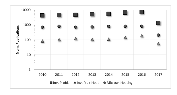
Figure 1
Publications in the last five years in the area of inverse problems, inverse problems in heat transfer and microwave heating. Scopus (2010-2017 (March)).
Source: Authors own creation

Hetmaniok [11] described the solution of an inverse problem, consisting of the estimation of the heat flux and the temperature profile in a binary alloy solidification process using Ant Colony Optimization. He assumed known temperature measurements at selected points. In a similar approach, Dasa [12] predicted thermal conductivity, variable conductivity coefficient, and surface heat transfer coefficient of an annular hyperbolic fin. For this task, he used a hybrid differential evolution optimization algorithm. In addition, his results showed that many feasible materials fulfilled the expected temperature distribution. In the same direction, a new proposal suggested by Mayedli et al. [13] applied the so-called ball spine algorithm concept for solving inverse heat conduction problems. According to the authors, these types of problems can be depicted as one with internal heat generation embedded within a solid medium with known temperature distribution. Their results show low computational time and high convergence rate. Adamczyk et al. [14] described an experimental technique combined with the solution of an inverse problem for estimating the thermal conductivity of isotropic and orthotropic materials. The classical Levenberg-Marquardt (LM) method for solving the minimization problem was used. According to the authors, this procedure exhibited good accuracy and high potential for several practical applications. Moaveni et al. [15] proposed an inverse model that could be used to determine the film heat transfer coefficient from the knowledge of two measured temperature values in the solid substrate. They conducted several numerical simulations to test its validity and found good agreement between the solutions of the direct problem and those of the inverse one. On the other hand, Huntul et al. [16] investigated inverse problems to reconstruct the time-dependent thermal conductivity. The Tikhonov regularization was employed to overcome the small errors in the input data. Using this method, the results were more stable and accurate.

Regarding the estimation of transient multidimensional heat flux distributions, Kant et al. [17] proposed a procedure for measuring surface temperature. The noticeable difference is that, for some cases, the heat flux profile was not required to be known beforehand, and no additional stabilization procedures were involved. Finally, Wróblewska et al. [18] proposed two strategies for solving an inverse conduction problem using the Discrete Fourier Transform (DFT). The first consisted of reducing the number of DFT components taken into account when determining the solution to the inverse problem. The second one was related to the regularization of the solution to the inverse problem. The authors claimed very good outcomes for this kind of approach.

Despite the vast amount of literature dealing with inverse problems, studies simultaneously involving microwave heating and estimating the properties of the material being irradiated are rather scarce. In the present article, we estimate thermal conductivity (k) and the volumetric heat capacity (pc) of a material irradiated with microwaves, in which the transient temperature field is known beforehand. We assume that these temperature values are taken with single and multiple sensors (i.e., 4) inserted in the solid sample. The resulting data under these settings are presented. The manuscript includes a brief description of the algorithms required for the solution of the inverse problem, along with the description and solution of the direct problem. After that, some of the more relevant results are presented and analyzed. Finally, we include the most relevant conclusions.

Materials and methods

In this section, a brief description of the LM, simulated annealing (SA) and genetic algorithms (GA) is presented. The reasoning behind this decision is that we want to prove three different strategies for the solution of this problem. The first one is the traditional method based on the gradient of the objective function; the other two are metaheuristics that have two different search principles. While the first one finds the solution based on a trajectory (similarly to LM), the second one does this based on a population. Next, we include the direct and inverse problem statements, along with the analysis of the solutions to the direct problem and a discussion of the temperature measurements. This section concludes with a discussion of the objective function used throughout this work.

Algorithm fundamentals

The LM method is a well-known iterative deterministic technique traditionally used for non-linear parameter estimation. The details are omitted for the sake of brevity, but they can be found in [1]. In contrast, Simulated Annealing (SA) is a probabilistic method for finding the global minimum of a cost function with several local minima [19]. This algorithm is inspired by the annealing of steel and ceramics. The underlying process first involves heating the material to excite its atoms. This allows them to move from their initial position (local minimum) to new ones. Afterwards, the material is cooled down, so that atoms can be recrystallized in a configuration with lower energy than the initial one (global minimum). The standard algorithm is concisely described as follows:

• Set an initial state s_k, and calculate its energy at a certain high initial temperature, where is the number of particles in the solution space.

• Randomly create a new state s¹_k that is a neighbor of the current state at the current temperature, and calculate its energy.

• If the energy of a neighbor state is better than the current solution s_k, replace the current solution with the new solution. If not, decide whether to move to the new state or not, depending on the current temperature. Then, decrease the temperature by a specified rate.

• If the temperature reaches the lower bound, stop the algorithm. If not, return to step b.

Similarly, Genetic Algorithm (GA) is a metaheuristic that uses the principles of selection and evolution to generate several solutions to a given global optimization problem. The standard algorithm is again concisely described as follows:

• Set an initial population of individuals.

• Evaluate the objective function.

• Choose the survivors, which are the best individuals. Individuals who do not survive are extinguished. Then, survivors are recombined and mutated to create a new generation.

• If the objective function reaches the lower bound, stop the algorithm. If not, return to step b.

A complete description of this algorithm appears in [20].

The model system

Within this work, we consider an isotropic and homogeneous solid sphere of radius (a), with constant density (p) and specific heat (c), for demonstrative purposes. The heat conduction equation expressed in spherical polar coordinates, assuming no variation for the (θ, ϕ) coordinates, as well as a constant heat generation rate q_0''' per unit volume at r=0, is given by equation 1, where α is the thermal diffusivity of the substance, is the thermal conductivity of the substance q_0''', is the heat flux generated in the solid at the point . is the temperature, and , and are the parameters of the spherical coordinates. The relationship between a and k is given by a=k/pc. The temperatures at its boundary and in the initial condition are assumed to be zero.

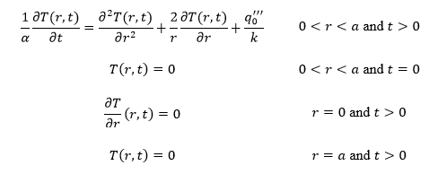[equation 1]

Direct problem statement

It is possible to describe the temperature distribution within the sphere homogeneously irradiated by microwaves. Here, we assume that all parameters of the above mathematical model are known, including initial and boundary conditions.

Inverse problem statement

The inverse problem aims at estimating the thermal conductivity and volumetric heat capacity of the material considered as an example. This requires knowledge of transient temperature measurements taken with single and multiple sensors (i.e., 4) located at exact positions within the sphere.

Direct problem solution

This problem already has an analytical solution and yields the temperature profile shown in equation 2,

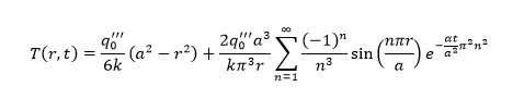[equation 2]

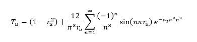
Prior to plotting equation 2, normalization for variables T, r, and t is carried out. New variables are denoted by T_u, r_u and , as shown in equation 3, where:

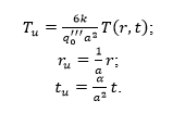[equation 4]

Figure 2 shows the normalized theoretical temperature within the sphere as a function of normalized radius and normalized time, as well as the temperature profile after a long time of irradiation. As expected, the temperature field is axisymmetric, with the maximum value at the center. In the first plot, the numbers on the curves represent the parameter t_u.

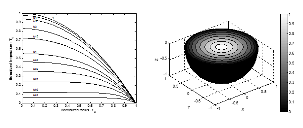
Figure 2
Normalized temperature (Tu) in the function of the normalized radius (ru) and normalized time (tu) for a sphere with constant internal heat generation q0'''. The numbers on the curves represent the normalized time (tu).
Source: Authors own creation.

Temperature measurements

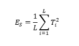
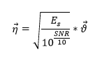
We use synthetic temperature values for simulating real measured values, to validate this approach for a microwave heating process analysis. As expected, the temperature measurements may contain random errors. Here, such errors are assumed to be additive, uncorrelated, and normally distributed with zero mean and constant standard deviation. Hence, we assume the basic standard statistical assumptions proposed by Beck as valid [1]. Consequently, a white Gaussian noise (AWGN) was added to the theoretical normalized temperature to construct synthetic ones. To do this, we have a theoretical temperature vector of length L whose components are Ti. We start by measuring the power of the signal (Es) in Watts [W], as defined by equation 5. Then, the noise vector ( ) can be found using equation 6, where SNR is the signal-to-noise-ratio given in [dB], and is a vector with Gaussian distributed random numbers of length . It is important to keep in mind that our vector is positive and real.

[equation 5]

[equation 6]

Finally, and as aforementioned, the measured temperature (synthetic temperature: a signal with white Gaussian noise) is obtained by adding white noise to the theoretical temperature values (original signal). In this work, the SNR per sample is fixed to 5, 10, 20 and 30 [dB]. Figure 3 shows an example of the normalized theoretical temperatures for a given position and time and the measured temperatures at normalized time t_{u =0.1}. If the SNR tends to zero, the temperature measurement distortion increases noticeably. In the remaining cases, the distortion becomes very small. For the sake of brevity in the text, vectors and are renamed Y and T.

Figure 3
An example of the measured (synthetic) temperature at with SNR=5, 10, 20 and 30 [dB]. The number on the curve represents the normalized time ().
Source: Authors’ own creation.

Objective function

The objective function (OF) that provides the minimum variance in an inverse problem is the ordinary least squares (OLS) norm given by equation 7, where and are vectors containing the synthetic (measured) and theoretical temperatures, respectively.

[equation 7]

n this work, we analyzed the following three cases:

Case a: Transient readings Y are taken from a single sensor.

Case b: Transient readings Y are taken from a single sensor where the standard deviation of the measurements is significant.

Case c: Transient readings are taken from multiple sensors (i.e., 4).

It is worth remarking that due to the simulated nature of this work, whenever the temperatures are labeled “measured,” they actually indicate simulated measurements generated by our model.

Case a: Single sensor with no variation in its measurements

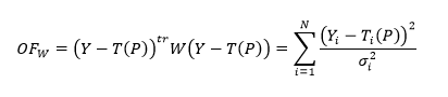
When transient readings Y are taken from a single sensor and the standard deviation of the measurements are similar, the objective function becomes equation 8, where N is the number of temperature measurements, and P is a vector containing the unknown parameters. Figure 4 shows the data of the normalized measured and theoretical temperatures for a sphere with internal heat generation, obtained with a single sensor at normalized radius r_u=0.5. To do this, we take 11 measurements at normalized times t_u=0.01, 0.02, 0.04, 0.06, 0.08, 0.1, 0.15, 0.2, 0.3, 0.4 and 1. The noise levels for the measured temperatures are 5, 10, 20 and 30 [dB]. In addition, we assume that those measurements do not have high variations. Therefore, each time we take the temperature at r_u=0.5 and at each t_u, the result is always going to be the same.

[equation 8]

Figure 4
Normalized measured and theoretical temperatures for the case when the measurements are taken with a single sensor with no variation in its measurements at normalized radius ru=0.5 and normalized time tu=0.01, 0.02, 0.04, 0.06, 0.08, 0.1, 0.15, 0.2, 0.3, 0.4 and 1. SNR is assumed to be 5, 10, 20 and 30 [dB] for the measured temperatures.
Source: Authors’ own creation

The median, the first and third quartiles, the extreme data and the outliers for the difference (error) between the normalized theoretical and measured temperatures at each noise level were calculated. Figure 5 shows these results. In the boxplot, the central mark is the median, the edges of the box are the first and third quartiles, the whiskers are the extreme data without considering the outliers and the outliers are the most extreme points (plotted individually). As we can see, at lower levels of SNR, the error increases considerably. The error of each data is obtained as follows:

[equation 9]

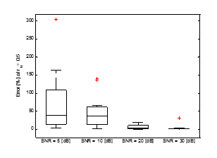
Figure 5
Boxplot of the error between the normalized theoretical and measured temperatures at each level of SNR. The central mark is the median, the edges of the box are the first and third quartiles, the whiskers are the extreme data without considering the outliers and the outliers are the most extreme points (plotted individually).
Source: Authors’ own creation.

Case b: Single sensor, with high variation in its measurements

When the standard deviations across measurements are quite different while using just one sensor, the objective function transforms into equation 10, where P is a vector containing the unknown parameters, and W is the diagonal weighting matrix. This matrix is defined in equation 11.

[equation 10]

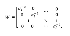[equation 11]

For this scenario, measurements at normalized radius r_u=0.5 were taken 30 times from just one sensor at 11 normalized times t_u=0.01, 0.02, 0.04, 0.06, 0.08, 0.1, 0.15, 0.2, 0.3, 0.4 and 1. Figure 6 shows the data of normalized measured (with high variation) and theoretical temperatures for a sphere with internal heat generation, obtained with a single sensor at normalized radius r_u=0.5. For brevity, only the noise level of 10 [dB] is shown in Table 1.

Figure 6
Normalized measured and theoretical temperatures for the case when the measurements were taken with a single sensor with high variation in its measurements at normalized radius ru=0.5 and normalized time tu=0.01, 0.02, 0.04, 0.06, 0.08, 0.1, 0.15, 0.2, 0.3, 0.4 and . SNR is assumed to be 5, 10, 20 and 30 [dB] for the measured temperatures. Each measurement was taken 30 times at each tu. The line at each tu represents the possible locations where the measured temperature can be
Source: Authors’ own creation.

Table 1

Mean and standard deviation of 30 measurements () with a single sensor at normalized radius and normalized time 0.01, 0.02, 0.04, 0.06, 0.08, 0.1, 0.15, 0.2, 0.3, 0.4 and 1. SNR is assumed to be 10 [dB] for the measured temperatures. is the theoretical temperature.

Source: Authors’ own creation.

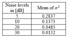
This table shows that the standard deviation at each normalized time is between 0.1067 and 0.1912. Now, in order to determine how the measurement is affected by the noise level, the mean of the standard deviations is calculated for each noise level. This parameter will tell us how data are dispersed. As an example, for a noise level of 10 [dB], the mean of the standard deviation is 0.1373. This procedure is repeated for 5 [dB], 20 [dB], and 30 [dB], and the results are shown in Table 2. As expected, we can see that as the noise level decreases, the standard deviation of Y increases.

Table 2

Mean of the measured temperature standard deviations for different noise levels.

Source: Authors’ own creation.

Case c: Multiple sensors (i.e., 4)

Finally, when transient readings are taken from multiple sensors, the objective function becomes equation 12, where M is the number of sensors for the experiment and P is a vector containing the unknown parameters. In this case, it is assumed that the standard deviation of the measurements is similar. Therefore, each time we take the temperature at each r_u and t_u each , the result is always going to be the same.

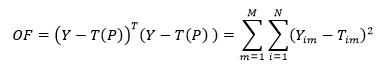[equation 12]

Figure 7 shows the data of the normalized measured and theoretical temperatures in a sphere with heat generation, obtained with four sensors at normalized radius and and at 11 normalized times 0.01, 0.02, 0.04, 0.06, 0.08, 0.1, 0.15, 0.2, 0.3, 0.4 and 1. The of the measured temperatures were 5, 10, 20 and 30 [dB]. For practical purposes, higher values of SNR mean better measurements.

Figure 7
Normalized measured and theoretical temperatures for the case where the measurements were taken with four sensors at normalized radius ru=0.3, 0.5, 0.7 and 1.0 and normalized time tu=0.01, 0.02, 0.04, 0.06, 0.08, 0.1, 0.15, 0.2, 0.3, 0.4 and 1. SNR is assumed to be 5, 10, 20 and 30 [dB] for the measured temperatures
Source: Authors’ own creation.

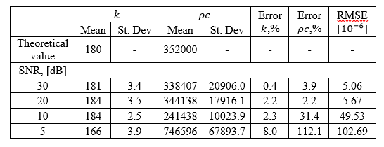
The statistical parameters considered here for the error between the normalized theoretical (T) and measured (Y) temperatures are the mean and the standard deviation. The results for the case of when the SNR is 30 [dB] are summarized in Table 3. The other cases of SNR are omitted because they exhibit the same pattern as presented below. In other words, as the noise level decreases, the error of Y increases.

Table 3

Some statistical parameters from the error data with four sensors between the normalized theoretical () and measured () temperature when the SNR is 30 [dB].

Source: Authors’ own creation

Results and analysis

A demonstrative example

We consider the microwave heating of an isotropic and homogeneous silicon carbide (SiC) sphere with constant density, thermal conductivity and specific heat p, k, and c respectively. Its diameter and internal heat generation rate at r=0 are 2 and 8000 [W/m³]. The temperature at its boundary is fixed at zero Celsius degrees. The goal is to estimate parameters and by solving the inverse problem. An Intel Core i5 computer running at 2.45 [GHz] with 6 [GB] of RAM and Windows operating system was used to run the tests. In addition, the initial conditions (IC) are located between 0.9 times the true value for the lower limit and 3 times for the higher limit for the LM cases, between 0.9 and 6 times for the SA cases and between 0.9 and 30 times for the GA cases. It is important to keep in mind that our work is based on normalized data. Therefore, parameters k and pc obtained through the algorithm are also normalized. However, the data shown within this section are related to their unnormalized equivalents.

Case a

Levenberg-Marquardt method (LM)

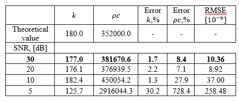
Now, we use the LM method to solve the inverse problem. The objective function is shown in equation 8. The expected values for k and p are , respectively. Therefore, in order to probe the LM method for parameter estimation, four datasets for the measured data are created, each one at a different noise level. In this case, the selected levels are 5 [dB], 10 [dB], 20 [dB] and 30 [dB]. Table 4 shows these parameters, as well as the error percentage of each parameter, compared to its theoretical value and the RMSE for the theoretical T and the estimated T_est temperatures. RMSE can be considered as a good measure of how accurately the model predicts the response. The RMSE is calculated using equation 13, where is the number of measurements at times t_i.

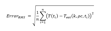[equation 13]

Table 4

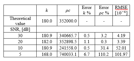
Estimated parameters and as well as their % of error and the RMSE of the profile temperature estimated.

Source: Authors’ own creation

Simulated Annealing (SA)

The objective function and noise levels are preserved since they depend on the problem and not on the solution approach. The parameters of the simulation are the initial temperature of 100 °C, the maximum number of objective function evaluation of 6000 and a termination tolerance of 1x10-6. We obtained these parameters after some preliminary testing with the OF to ensure the correct operation of the algorithm. However, for the sake of brevity, these data are not shown. Table 5 shows the estimated parameters (k and pc), as well as the percentage of error, when compared to the expected theoretical value. The data show that the error sits at below 3.9% for noise levels under 20 [dB].

Table 5

Estimated parameters and as well as their % of error and the RMSE of the profile temperature estimated.

Source: Authors’ own creation.

Genetic Algorithm (GA)

Finally, we repeat the procedure using a GA. Simulations were carried out using 100 generations, a crossover fraction of 0.8, a migration fraction of 0.2, a termination tolerance of 1x10^-6 and a population of 400. We also obtained these parameters via preliminary testing. Again, these data are omitted for the sake of brevity. This time, the error margins are under 3.5% for noise levels below 20 [dB].

Table 6

Estimated parameters and as well as their % of error and the RMSE of the profile temperature estimated.

Source: Authors’ own creation.

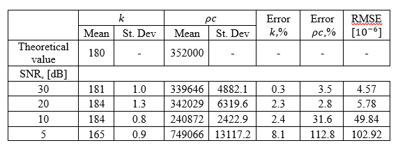
Case b

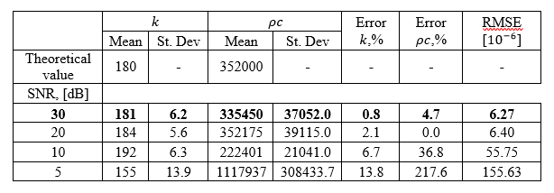
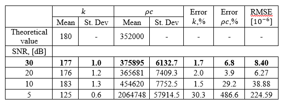
Repeating the procedure for case b requires using the objective function given in equation 10. Table 7 to Table 9 show the estimated parameters ( and), as well as the error percentages, when compared to the expected theoretical value and the RMSE. As foreseeable for the three algorithms, a high RMSE value indicates a considerable discrepancy between the predicted values and the estimated ones.

Levenberg-Marquardt method

Table 7 shows the estimated data, the error percentage compared to the expected theoretical value, and the RMSE. Although the RMSE value for 30 [dB] is a little higher than that for SNR of 20 [dB], the estimated conductivity is closer to the expected one. The opposite is observed for the estimated parameter under the same conditions.

Table 7

Estimated parameters and as well as their % of error and the RMSE of the profile temperature estimated.

Source: Authors’ own creation.

Simulated annealing

Table 8

Estimated parameters and as well as their % of error and the RMSE of the profile temperature estimated.

Source: Authors’ own creation.

Genetic Algorithms

Table 9

Estimated parameters and as well as their % of error and the RMSE of the profile temperature estimated

Source: Authors’ own creation.

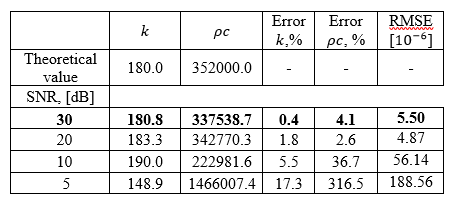
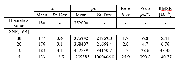
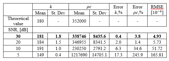
Case c

This final case implies the use of the objective function shown in 12. Table 10 to Table 12 include some of the most important results. To compare the simulation results, we used the RMSE. For all of the results shown in these tables dealing with SNR values lower than 20, the RMSE reached considerably higher values, indicating a substantial disagreement between the predicted temperatures and the estimated ones. This behavior has an evident negative impact on the estimated parameters. Nonetheless, Simulated Annealing reached the lowest RMSE for SNR = 30 [dB], when compared with LM and GA.

Levenberg-Marquardt method

Table 10

Estimated parameters and as well as their % of error and the RMSE of the profile temperature estimated.

Source: Authors’ own creation.

Simulated annealing

Table 11

Estimated parameters and as well as their % of error and the RMSE of the profile temperature estimated.

Source: Authors’ own creation.

Genetic Algorithms

Table 12

Estimated parameters and as well as their % of error and the RMSE of the profile temperature estimated.

Source: Authors’ own creation.

Algorithm performance

Comparing the performances of all three algorithms requires a common metric. Thus, the number of iterations, as well as the number of function evaluations, was measured. For genetic algorithms, the number of generations was analyzed instead of the number of iterations. The data are shown in Table 13 for LM and SA. However, in the case of GA, the detailed performance results are omitted because the total number of generations and the number of function evaluations are 51 and 201800, respectively, in all cases. From the performance results, it is found that LM is slightly faster than the other two. Nonetheless, this method is very dependent on the location of initial conditions. Thus, an improper selection may lead to a solution located far from the optimum, or to no solution at all. Similarly, it is evident that SA yields data close to the expected optimal. Its main advantage lies in improving the search of the solution domain of LM. Therefore, it is somewhat independent of initial conditions. The remaining approach, i.e., GA, also yields acceptable results and improve the search of the solution domain of the two previous methods. However, GA requires more function evaluations than the other two approaches and thus takes longer to converge.

Table 13

Other parameters derived from the analysis of the LM method such as the number of iterations and the number of function evaluations employed by the algorithm.

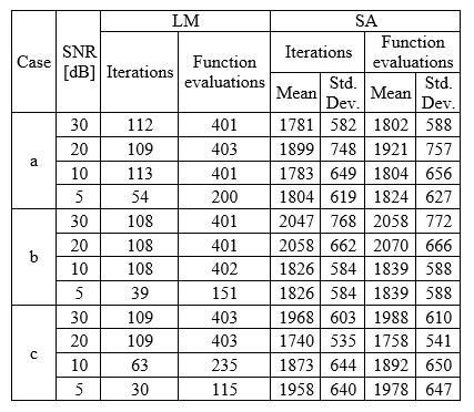
Source: Authors’ own creation.

Conclusions

In this article, we analyzed an alternative technique for estimating, in real-time, the thermal conductivity and the volumetric heat capacity of a material heated by microwaves. It was found that all three selected optimization algorithms could be used for this purpose if the measurements have low noise levels. This means that the estimation procedure is highly dependent on the quality of both the experimental design and the electronic instrumentation used. If both requirements are satisfied, it is possible to estimate these parameters on-line without the need for an additional experimental setup. For the case of the algorithms, their behaviors differed in features such as the dependence on initial conditions and the number of required function evaluations. Weighing these differences lead to the consideration of the SA algorithm as advantageous among all three approaches, especially for a real situation (case c) when transient temperature readings are taken from multiple sensors (i.e., 4). However, by the nature of the GA algorithm, it improves six times the search space solution of the SA algorithm. Likewise, it was observed that normalizing the objective function for data with high standard deviations helps to produce results close to the optimum, in spite of the said dispersion. In a future work, it is necessary to include more internal heat generation models and boundary conditions. Moreover, hybrid methods should be tried in order to take advantage of each algorithm’s strength, i.e., a hybrid between SA and GA. Lastly, other modern, stable and metaheuristic algorithms with good performances should be tried, such as PSO.

Acknowledgment

The authors express their gratitude for the financial support given by the Universidad Industrial de Santander.

References

[1] M. J. Colaço, H. R. B. Orlande, and G. S. Dulikravich, “Inverse and optimization problems in heat transfer,” J. Brazilian Soc. Mech. Sci. Eng., vol. 28, no. 1, pp. 1–24, 2006.

[2] M. A. Ahmadi, M. Ebadi, A. Shokrollahi, and S. M. Javad Majidi, “Evolving artificial neural network and imperialist competitive algorithm for prediction oil flow rate of the reservoir,” Appl. Soft Comput. J., vol. 13, no. 2, pp. 1085–1098, 2013.

[3] M. A. Ahmadi, R. Soleimani, M. Lee, T. Kashiwao, and A. Bahadori, “Determination of oil well production performance using artificial neural network (ANN) linked to the particle swarm optimization (PSO) tool,” Petroleum, vol. 1, no. 2, pp. 118–132, 2015.

[4] M. A. Ahmadi, M. Zahedzadeh, S. R. Shadizadeh, and R. Abbassi, “Connectionist model for predicting minimum gas miscibility pressure: Application to gas injection process,” Fuel, vol. 148, pp. 202–211, 2015.

[5] M. A. Ahmadi, B. Pouladi, Y. Javvi, S. Alfkhani, and R. Soleimani, “Connectionist technique estimates H2S solubility in ionic liquids through a low parameter approach,” J. Supercrit. Fluids, vol. 97, pp. 81–87, 2014.

[6] A. Shafiei, M. A. Ahmadi, S. H. Zaheri, A. Baghban, A. Amirfakhrian, and R. Soleimani, “Estimating hydrogen sulfide solubility in ionic liquids using a machine learning approach,” J. Supercrit. Fluids, vol. 95, pp. 525–534, 2014.

[7] M. A. Ahmadi and M. Ebadi, “Evolving smart approach for determination dew point pressure through condensate gas reservoirs,” Fuel, vol. 117, no. PARTB, pp. 1074–1084, 2014.

[8] P. Duda, “Solution of Inverse Heat Conduction Problem using the Tikhonov Regularization Method,” J. Therm. Sci., vol. 26, no. 1, pp. 60–65, 2017.

[9] M. Cui, K. Yang, X. Xu, S. Wang, and X. Gao, “A modified Levenberg–Marquardt algorithm for simultaneous estimation of multi-parameters of boundary heat flux by solving transient nonlinear inverse heat conduction problems,” Int. J. Heat Mass Transf., vol. 97, pp. 908–916, 2016.

[10] M. Shusser, “Using a Double Genetic Algorithm for Correlating Thermal Models,” Heat Transf. Eng., vol. 37, no. 10, pp. 889–899, 2016.

[11] E. Hetmaniok, “Solution of the two-dimensional inverse problem of the binary alloy solidification by applying the Ant Colony Optimization algorithm,” Int. Commun. Heat Mass Transf., vol. 67, pp. 39–45, 2015.

[12] R. Dasa, “Identification of materials in a hyperbolic annular fin for a given temperature requirement,” Inverse Probl. Sci. Eng., vol. 24, no. 2, pp. 213–233, 2016.

[13] P. Mayeli and H. Nili-Ahmadabadi, M Besharati-Foumani, “Inverse shape design for heat conduction problems via the ball spine algorithm,” Numer. Heat Transf. Part B Fundam. An Int. J. Comput. Methodol., vol. 69, no. 3, pp. 1–21, 2016.

[14] W. Adamczyk, R. Białecki, and T. Kruczek, “Retrieving thermal conductivities of isotropic and orthotropic materials,” Appl. Math. Model., vol. 40, no. 4, pp. 3410–3421, 2016.

[15] S. Moaveni and J. Kim, “An inverse solution for reconstruction of the heat transfer coefficient from the knowledge of two temperature values in a solid substrate,” Inverse Probl. Sci. Eng., pp. 1–25, 2016.

[16] M. J. Huntul, D. Lesnic, and M. S. Hussein, “Reconstruction of time-dependent coefficients from heat moments,” Appl. Math. Comput., vol. 301, pp. 233–253, 2017.

[17] M. Kant and P. Rudolf von Rohr, “Determination of surface heat flux distributions by using surface temperature measurements and applying inverse techniques,” Int. J. Heat Mass Transf., vol. 99, pp. 1–9, 2016.

[18] A. Wróblewska, A. Frąckowiak, and M. Ciałkowski, “Regularization of the inverse heat conduction problem by the discrete Fourier Transform,” Inverse Probl. Sci. Eng., vol. 24, no. 2, pp. 195–212, 2016.

[19] E. Aarts, J. Korst, and W. Michiels, “Simulated Annealing,” in Search Methodologies Introductory Tutorials in Optimization and Decision Support Techniques, 2nd ed., 2014, pp. 265–285.

[20] K. Sastry, D. E. Goldberg, and G. Kendall, “Genetic Algorithms,” in Search Methodologies Introductory Tutorials in Optimization and Decision Support Techniques, 2nd ed., 2014, pp. 93–118.

Notes

Author notes