1. Introduction

Multiphase flows are present in processes in the petrochemical industry, which has focused a significant portion of its resources on optimizing the production and transportation of oil and gas. In light of the development of Industry 4.0, the oil industry has focused its attention on implementing technologies for the characterization of multiphase flows [1], where the goal is to classify the type of multi-flow through the pipes. To do this, a detailed description of the different spatial distributions of the phases (liquid or gas) is required, known as regimes or flow patterns, which refer to the fluid configuration within the pipe [2, 3]. Predicting the behavior of flow patterns, taking into account the phases in which the fluids are found, whether solid, liquid, or gas, allows for accurate estimates of process parameters, optimization of infrastructure, personnel use, and reduction of operational costs [4].

Research has been conducted on two-phase liquid-liquid flow studies to understand their behavior under various conditions, particularly the mixture of oil and water [5]. This type of flow is dependent on numerous variables such as the geometry of the pipe (length, inclination, material, diameter), as well as the properties present in the mixture (surface tension, viscosity, and density), and the volume flows [6]. The estimation of pressure gradients and fluid volume fractions are directly linked to the determination of flow patterns within a pipeline [5]. The volume fraction is a dimensionless measure that allows us to know the quantity of each component of the mixture in a multiphase system, which consists of dividing the volume of the component of the system over the total volume of the mixture [7]. Also, the calculation of the volume fraction is relevant since it can be used to determine the amount of water and oil inside a well, and to identify zones with high volume fractions of the fluids to be extracted [8].

In search of greater accuracy and flexibility in the analysis of industrial process data in real-time, improvements in connectivity have been implemented through the use of technologies such as the Internet of Things (IoT), cloud storage, robotics, and artificial intelligence (AI) [9], [10]. Artificial intelligence (AI) can process large amounts of data and obtain accurate predictions about future process conditions [11]. In this way, greater accuracy in modeling system operation is achieved and the understanding of the phenomena related to fluid transport in multiphase flows is improved [12],[15].

Utilizing artificial neural networks (ANN) proves valuable in addressing challenges encountered in controlling processes involving multiphase flows. The efficacy of ANNs lies in their capability to discern intricate behavioral patterns within extensive datasets [16], thereby enabling the resolution of issues associated with characterizing two-phase systems [17], [18]. The goal of machine learning is to create computational models and methods that, without the need for specialized programming, enable machines to learn from data and prior experiences [19]. Three steps make up the learning process: training, validation, and testing. The model is fed a set of data, including sample inputs and expected outputs, during the training phase. In this process, an optimizing algorithm is used by the algorithm to modify the internal parameters to reduce the error between the predicted and expected results [19]. To ensure that the model produces appropriate values for the output and is not overfitted to the training data, model validation is subsequently carried out by analyzing a data set that was not used in training [20]. Once the model has been trained and validated, it is tested on a completely unseen dataset called the test set. Testing ensures that the model can generalize well to new, unseen data and provides an estimate of its real-world performance. Machine learning models can be supervised, unsupervised, or use reinforcement learning, depending on the requirements of the application [21]. Supervised models are used to predict an output from input data, while unsupervised models are used to identify patterns in data without requiring prior outputs [22]. Reinforcement learning focuses on learning decision-making through interactions with the environment [21]. Deep learning is a machine learning technique based on neural networks with multiple layers that allows processing large datasets without clear structuring, such as images, voice, text, and video, to identify complex patterns and relationships that are not easily detected by humans [23]. In the oil and gas industry, deep learning is used for production process optimization, predictive maintenance, equipment monitoring, prediction of oil and gas reserves, and processing and analysis of satellite images related to oil exploration and production [24].

Recurrent neural networks (RNNs), a type of machine learning model that can remember previously worked information and use it to make future predictions, are used in the processing of data streams, such as text and audio [25]. The architecture of RNNs behaves in such a way that the output of one neuron is used as input to the next, allowing information to flow through time and behavioral patterns to be captured in complex temporal sequences [25]. However, the performance of RNNs faces difficulties in deep network training due to the disappearance of the gradient. Therefore, a variant of RNNs called LSTM (Long Short Term Memory) networks was developed that solves this problem [26]. LSTM networks differ from RNNs in their structure, as they function as gates that control the flow of information by deciding what information is important to remember and what information is not relevant [26]. LSTM networks are composed of memory cells connected by input, output, and forgetting gates [27]. The function of these gates is to control the storage of information in each cell such that the network learns to remember only information relevant to the process and discards unimportant information [28]. LSTM networks have been very successful in various applications, including natural language processing, behavioral pattern regression, and image classification, thanks to their ability to work with long and complex data sequences [28].

The modeling discussed typically employs CFD with RANS models, which are computationally efficient. However, these methods have limitations, particularly when dealing with complex geometries and highly transient flows. While RANS models provide time-averaged solutions and are less computationally intensive compared to more detailed simulations like DNS (Direct Numerical Simulation), they often fail to capture fine-scale turbulence and transient phenomena accurately [29], [30]. In this context, the development of LSTM models presents a significant opportunity. LSTM networks, designed for handling sequential data and capturing temporal dependencies, offer the potential to predict flow dynamics in real-time with a higher degree of accuracy [30]. These models can serve as a complementary or alternative approach to traditional CFD, potentially reducing computational costs while enhancing predictive capabilities [31]. Recent studies have demonstrated that integrating LSTM models into CFD frameworks can significantly improve the accuracy of flow predictions, particularly in complex flow scenarios [30], making them a powerful tool for industrial applications where both precision and efficiency are critical.

This research primarily focuses on studying the behavior of liquid-liquid two-phase flow, specifically involving water and oil. We consider key characteristics such as substance viscosities, pressure differentials within the pipeline, and volume fractions. The objective is to explore the feasibility of employing Long Short-Term Memory (LSTM) neural networks to estimate the volume fraction in a horizontal pipe where both oil and water are present. Assessing the accuracy of the prediction model is crucial, achieved by comparing outcomes obtained through training different neural network architectures. This approach aims to leverage artificial intelligence to enhance the understanding and prediction of fluid behavior.

2. Materials and Methods

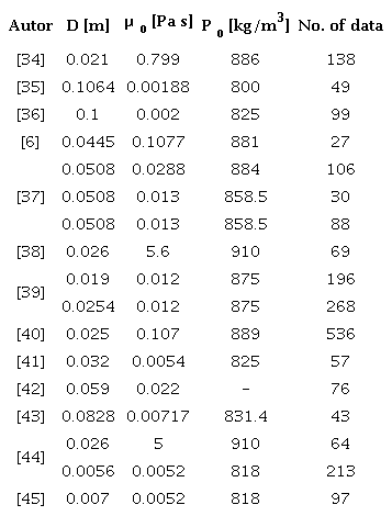
An analysis of experimental information obtained from previous research [11], [32], [33], investigating the behavioral characteristics of a two-phase fluid, was conducted. In this study, information collected from 13 authors focused on the behavior of a mixture of oil and water in horizontal piping, and 17 different schemes were presented, see Table 1. The dataset comprises a total of 2,156 experimental data points gathered from previous research.

Table 1
Summary of collected database

Fuente: [11], [32], [33].

Autor	D [m]	μo [Pa s]	Po [kg/m3]	No. of data
[34]	0.021	0.799	886	138
[35]	0.1064	0.00188	800	49
[36]	0.1	0.002	825	99
[6]	0.0445	0.1077	881	27
[37]	0.0508	0.0288	884	106
	0.0508	0.013	858.5	30
	0.0508	0.013	858.5	88
[38]	0.026	5.6	910	69
[39]	0.019	0.012	875	196
	0.0254	0.012	875	268
[40]	0.025	0.107	889	536
[41]	0.032	0.0054	825	57
[42]	0.059	0.022	-	76
[43]	0.0828	0.00717	831.4	43
[44]	0.026	5	910	64
	0.0056	0.0052	818	213
[45]	0.007	0.0052	818	97

In addition to the analysis of the experimental data, 216 experiments were systematically designed and conducted to explore the influence of key parameters on the predictive model's performance. These experiments did not strictly follow a Design of Experiment (DoE) approach but were structured to vary parameters such as the number of neurons, learning rate, batch size, and the number of epochs in a controlled manner. This approach allowed for a comprehensive evaluation of each variable's individual impact and the interactions between them, providing insights into the optimal configuration for predicting the volume fraction in a two-phase flow.

The collected variables include the internal diameter of the pipe, D, oil viscosity, ß₀, oil density, p₀ which are critical in determining the flow characteristics and are used in conjunction with other parameters like surface velocities and volume fractions of oil and water.

2.1. Neural network design

In order to structure the network effectively, preprocessing of the data is essential. This was accomplished using Python software, utilizing libraries such as Pandas and Matplotlib for data analysis and visualization [46]. The appropriate process of organization and preprocessing of the raw data was fundamental to achieve an adequate transformation and cleaning of the data. Since the information was in different scales, a normalization process of the database was performed to compare them properly and avoid extreme values dominating the analysis.

The data set was separated in such a way that the input vector with the required information and the output vector could be obtained. In this process, the input vector X was specified with a dimension of five rows, excluding the data of the volume fraction of the oil:

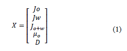
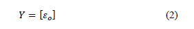
The surface velocities of oil, J₀ , and water, J_w , the sum of the surface velocities of oil and water, J₀+_w , and the volume fraction of both oil, ε₀, and water, ε_w, in the fluid were crucial parameters in the modeling process. Similarly, the process of organizing the output vector Y of the system was carried out, consisting of the selection of the data with the volume fraction of the oil:

Once the correct vectorization of the information was achieved, the data was segmented for training and testing the system, using a proportion of 80% and 20% of the total information, respectively, adhering to conventional practices that promote effective learning and ensure robust model generalization. These values were selected to maintain the balance of the system. Therefore, the training data consisted of 1724 independent records, while the test data consisted of 432 records to evaluate model performance.

For this study, the use of a recurrent neural network (RNN) is proposed to develop a predictive model of oil and water volume fraction in a two-phase flow. The RNN architecture is capable of processing and predicting data sequences thanks to its memory function and feedback connections, which differentiates it from conventional neural networks.

Long Term Memory Networks (LSTM) are a special variant of Recurrent Neural Networks (RNN), designed to achieve better prediction of long-term data sequences [46], [47], [48]. This is due to the presence of memory cells that update their internal information in each cycle, allowing a better retention of relevant information throughout the sequence. In this type of model, the network is required to have at least one hidden layer to achieve a good prediction. The neurons in each hidden layer use the backpropagation process to adjust the synaptic weights of the neural connections to minimize the prediction error in the network output. This adjustment is performed from the output layer to the input layer. After the adjustment of the synaptic weights, a ReLu-type transfer function is used to improve the accuracy in determining the desired output value. Mathematically, the net input function I(t) can be expressed as:

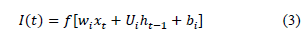
Where f represents the activation function ReLu, w_¿ the matrix of synaptic weights, x_t the input at time t, U_t the weight matrix of the previous output, h_t-1 the output of the neuron at time t - 1, and b_t the bias vector.

The appropriate selection of activation functions was a crucial step in the development of the model.

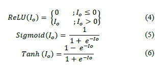
Considering the nature of the dataset and the focus of this study, we chose the Rectified Linear Unit (ReLU), Sigmoid (Sigmoid), and Hyperbolic Tangent (Tanh) as our activation functions.

The operational ranges for ReLU and Sigmoid are [0,1], while for Tanh, it is [-1,1], which adequately suits the needs for analyzing our data. These functions are defined as:

The output function I₀ is described in terms of the flow rates of oil Jo and water Jw, the sum of the surface velocities of oil and water J_0+w , and the volume fraction of both oil ε₀ and water ε_w within the fluid. The output function represents the result obtained after the neuron has completed its processing and will be used as input to the next neuron in the next hidden layer. The proposed model was implemented using Python libraries tailored for machine learning and data processing, including Sklearn, TensorFlow, and Keras. Figure 1 shows the overall architecture of the structured neural network.

In total, 216 experiments were conducted to fine-tune critical hyperparameters such as the number of epochs, learning rate, batch size, and the configuration of hidden layers. The neurons in the hidden layers varied across four configurations: 25, 50, 100, and 150, typically arranged in one to three hidden layers. The epochs used in the experiments were 10, 20, and 50, learning rates were either 0.1 or 0.2, and batch sizes were adjusted to 1 or 3. For the hidden layer, ReLU activation functions were chosen to efficiently handle the issue of vanishing gradients. In the output layer, ReLU, sigmoid, and Tanh functions were utilized to normalize the model's outputs within a range of 0 to 1, important for accurately representing the volumetric fraction. The optimizers ADAM and RMSprop were tested, ADAM proved superior due to its ability to adapt weights through adaptive gradients effectively, while RMSprop was beneficial for its capability to adjust the learning rate based on an average of recent gradients, enhancing convergence in recurrent models like the LSTM. This detailed approach in optimizing hyperparameters significantly enhanced the model's accuracy in predicting biphasic flows and provided valuable insights into the optimal configuration of hyperparameters for its application.

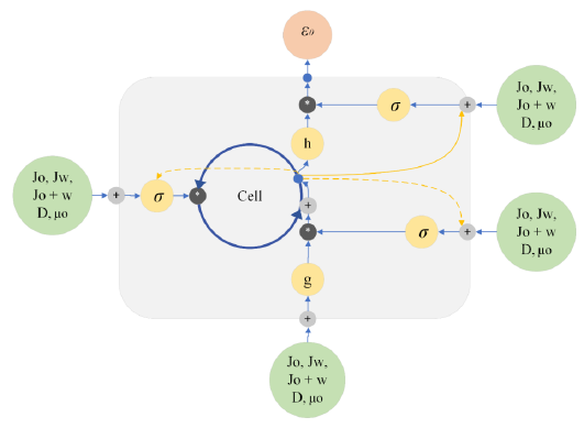
Figure 1
Schematic representation of the artificial neural network structure used.

2.2. Model validation and error analysis

In the model training process, various errors may emerge that can significantly influence the overall performance and accuracy of the predictive model. These errors are often associated with several key factors in the architecture and training protocol of the neural network. One such factor is the number of neurons in each layer, which can affect the ability of the model to generalize from the training data to unseen data. Additionally, the choice of optimizer, whether ADAM, SGD, or others, plays a critical role in how effectively the model converges to a minimum error during training.

The activation functions selected, such as ReLU, Sigmoid, or Tanh, also impact the learning dynamics of the model. Each function has specific characteristics that can either aid or hinder the training process depending on the nature of the data being processed. Moreover, the volume of data available for training is crucial, as insufficient data can lead to overfitting, where the model performs well on training data but poorly on new, unseen data.

To quantify and monitor these errors, we utilized the mean squared error (MSE) as a primary evaluation metric, which evaluates the average squared difference between the estimated values and the actual value, and reads:

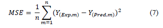
Where n represents the total number of input data, Y(_Exp) the experimental value of the output, and Y(_Pred) the value obtained with the intelligent model.

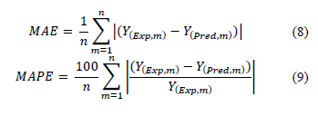
In addition to using the mean square error (MSE) to evaluate model accuracy, it is also proposed to use the mean absolute error (MAE) and the mean absolute percentage error (MAPE). The inclusion of these parameters allows for comprehensive validation of information, facilitates result comparison, and aids in identifying configurations with superior accuracy.

3. Results

Based on the parameters discussed in Section 2, which describes the methodology for evaluating model performance and determining optimal configurations, we present our findings segmented by the number of neurons in the hidden layers. Accordingly, we conducted a series of 216 experiments to analyze the performance of the system. This involved a comparative assessment of the model's outputs against a designated set of validation data, reserved specifically for testing purposes.

The different configurations implemented in the system generate distinctive behaviors in the results. Notice that one of the modified parameters was the maximum number of epochs of the system, which was set at 50. The results for test 4 which for 50 epochs showed the lowest value of the MSE, with 6.54E-06, and MAPE of 3.37%. Comparatively, test 35 conducted over 20 epochs yielded an MSE of 3.56E-05 and a MAPE of 3.02%. Despite the slight performance variance under 0.4% between these two setups, the longer epoch length increased computational time by approximately 4 to 5 minutes. Consequently, it was decided to lower the number of epochs to 20 and, if necessary, to 10 in future tests to optimize both performance and computational efficiency.

Additionally, during the experiments, it was observed that configurations with a larger number of neurons and a greater number of epochs required significantly longer processing times. For example, configurations with 150 neurons and 50 epochs showed an improvement in model accuracy but at a considerably higher computational cost, increasing training time by 50% compared to configurations with 20 epochs. This trade-off between computational cost and accuracy emphasizes the importance of finding an optimal balance, particularly in scenarios where computational resources are limited or real-time processing is required.

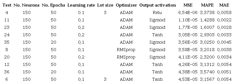
Table 2 shows the 10 configurations with the best MSE, structured in their hidden layers with 150 neurons. The results show that with this type of configuration an MSE of 6.5416E-06 can be achieved, as well as an MAE of 0.0058 and an MAPE of 3.3738%.

In Table 3, the performance of the model with an architecture of 100 neurons in its hidden layer and with 20 epochs presents an MSE of 6.38E-05, compared to the 3.56E-05 presented in Table 2. Similarly, the MAPE presents a performance of 4.08% and an MAE of 0.0048, obtaining a lower performance than the configurations presented in Table 2.

Table 2
Model performance varying the main parameters, and using 150 neurons, for the 10 configurations with the best MSE

Test	No. Neurons	No. Epochs	Learning rate	Lot size	Optimizer	Output activation	MSE	MAPE	MAE
4	150	50	0.1	3	ADAM	Relu	6,54E-06	3,3738	0,0058
11	150	50	0,1		ADAM	Sigmoid	1,10E-05	1,4288	0,0022
23	150	50	0,2		ADAM	Sigmoid	1,77E-05	1,6007	0,0028
24	150	50	0,2		ADAM	Tanh	3,05E-05	2,9303	0,0033
35	150	20	0,1		ADAM	Sigmoid	3,56E-05	3,0250	0,0045
8	150	50	0,1		RMSprop	Sigmoid	3,58E-05	3,2018	0,0038
20	150	50	0,2		RMSprop	Sigmoid	4,11E-05	2,3200	0,0034
12	150	50	0,1		ADAM	Tanh	4,26E-05	3,1312	0,0054
36	150	20	0,1		ADAM	Tanh	4,38E-05	3,5740	0,0051
6	150	50	0,1	3	ADAM	Tanh	4,53E-05	3,1567	0,0054

Table 3
Model performance with a full variation of main parameters, using 100 neurons

Test	No. Neurons	No. Epochs	Learning rate	Lot size	Optimizer	Output activation	MSE	MAPE	MAE
78	100	20	0,1	3	ADAM	Tanh	6,38E-05	4,0851	0,0048
77	100	20	0,1	3	ADAM	Sigmoid	6,53E-05	3,6244	0,0054
81	100	20	0,1	1	RMSprop	Tanh	6,71E-05	3,3238	0,0045
89	100	20	0,2	3	ADAM	Sigmoid	6,92E-05	2,9174	0,0050
83	100	20	0,1		ADAM	Sigmoid	8,03E-05	4,2026	0,0058
94	100	20	0,2		ADAM	Relu	8,60E-05	3,9164	0,0067
80	100	20	0,1		RMSprop	Sigmoid	9,11E-05	3,6893	0,0061
82	100	20	0,1		ADAM	Relu	1,06E-04	5,8229	0,0076
107	100	10	0,1		ADAM	Sigmoid	1,12E-04	4,9202	0,0089
104	100	10	0,1		RMSprop	Sigmoid	1,25E-04	4,5328	0,007

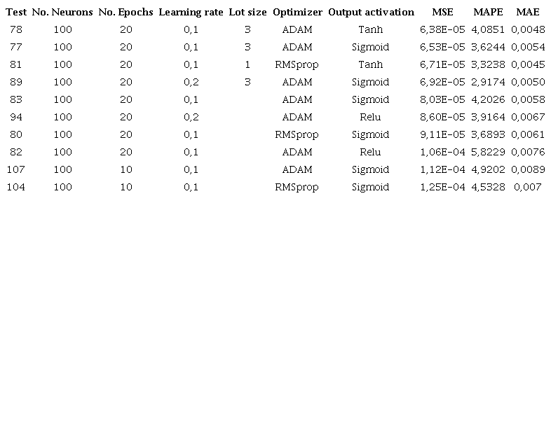
Table 4 shows the results for the 10 configurations with the best MSE, considering 50 neurons in the hidden layer. The system presents a behavior where, in comparison with Table 3 the values of the MSE and MAPE present an increase, reaching in this case 5.59E-05 and 3.33%, respectively, while the MAE remains stable. This comparison still does not exceed the performance presented in Table 2. On the other hand, notice that the model has better performance in this configuration when using a batch size of 1 as well as a learning rate of 0.1 by performing 20 epochs in the process and implementing. On the other hand, notice that the model has better performance in this configuration when using a batch size of 1 as well as a learning rate of 0.1 by performing 20 epochs in the process and implementing activation functions such as sigmoid and hyperbolic.

Table 4
Model performance varying the main parameters, using 50 neurons, and for the 10 configurations with the best MSE

Test	No. Neurons	No. Epochs	Learning rate	Lot size	Optimizer	Output activation	MSE	MAPE	MAE
131	50	20	0,1	1	ADAM	Sigmoid	5,59E-05	3,3392	0,0048
128	50	20	0,1	1	RMSprop	Sigmoid	6,94E-05	3,6845	0,0047
132	50	20	0,1	1	ADAM	Tanh	7,86E-05	6,2786	0,0062
129	50	20	0,1	1	RMSprop	Tanh	9,38E-05	5,3622	0,0063
137	50	20	0,2	3	ADAM	Sigmoid	9,83E-05	3,5328	0,0059
125	50	20	0,1	3	ADAM	Sigmoid	1,00E-04	4,1487	0,0074
142	50	20	0,2	1	ADAM	Relu	1,06E-04	4,0291	0,0074
156	50	10	0,1	1	ADAM	Tanh	1,10E-04	3,9565	0,0074
153	50	10	0,1	1	RMSprop	Tanh	1,26E-04	3,4953	0,0078
127	50	20	0,1	1	RMSprop	Relu	1,26E-04	5,1179	0,0077

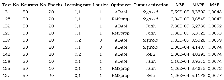
Table 5 shows the results for configurations with a structure of 25 neurons in its hidden layer. It shows a decrease in the performance of the MSE and MAE with respect to the previous configurations, presenting an error of 8.2504E-05 and 0.0063, respectively. Regarding the analysis of the MAPE, an improvement can be seen with respect to Table 4 since it presents a value of 3.1885% compared to 3.3392% of the previous result, showing an improvement of 0.15%.

Table 5
Model performance varying the main parameters, using 25 neurons, and for the 10 configurations with the best MSE

Test	No. Neurons	No. Epochs	Learning rate	Lot size	Optimizer	Output activation	MSE	MAPE	MAE
191	25	20	0,2		ADAM	Sigmoid	8,25E-05	3,1885	0,0063
189	25	20	0,2		RMSprop	Tanh	8,57E-05	2,651	0,006
175	25	20	0,1		RMSprop	Relu	1,31E-04	5,431	0,0078
192	25	20	0,2		ADAM	Tanh	1,41E-04	4,5988	0,0083
188	25	20	0,2		RMSprop	Sigmoid	1,67E-04	4,3604	0,0095
176	25	20	0,1		RMSprop	Sigmoid	1,70E-04	4,7803	0,0095
171	25	20	0,1		RMSprop	Tanh	1,89E-04	5,8035	0,0098
203	25	10	0,1		ADAM	Sigmoid	2,05E-04	6,3683	0,0096
178	25	20	0,1		ADAM	Relu	2,07E-04	7,7444	0,0101
173	25	20	0,1	3	ADAM	Sigmoid	2,23E-04	6,0608	0,0092

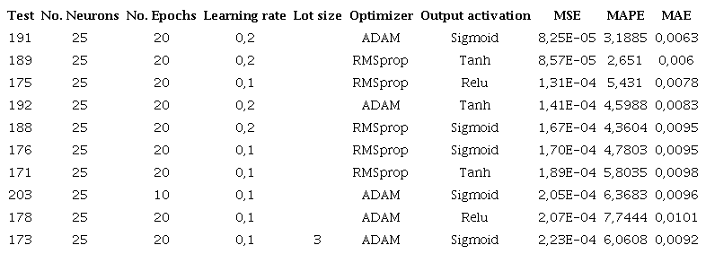
Figure 2 shows the behavior of the mean square error and its relationship with the varying parameters: number of neurons and number of epochs in the system. Higher number of neurons showed lower values of MSE. Lower values of epochs showed higher values of MSE. Note that during the development of the 216 tests, there was no marked trend in the behavior of the system, and a more detailed analysis of the performance of the model is required. To perform a more detailed analysis of the system performance results, it was proposed in Figure 3 to organize the MSE values from smallest to largest and compare them in the number of neurons to review the correlation between them and show the influence of this parameter on the model performance. Notice that with configurations with 150 and 100 neurons, better MSE performances are achieved in the system.

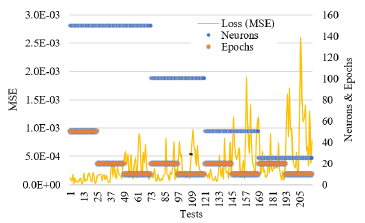
Figure 2
MSE behavior related to the number of neurons and epochs in the system.

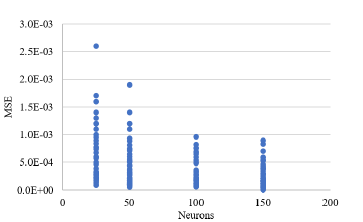
Figure 3
Correlation between the number of neurons in the hidden layer and the MSE of the system.

Figure 4 shows the correlation between the number of neurons implemented in the system and the result of the mean absolute error (MAE) metric. It can be seen that, unlike the results presented by the MSE, which were much more segmented, in this case, the values are very similar. However, it is possible to see a small difference between the systems with 150 and 100 neurons and those with 50 and 25, respectively.

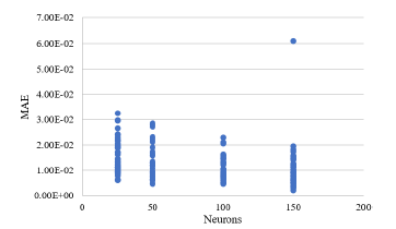
Figure 4
Variation of the mean absolute error (MAE) considering the number of epochs.

This analysis supports what was mentioned in Table 2. MAPE results were compared with the number of neurons present in the system, as shown in Figure 5. Similar to previous results, the configurations with 150 and 100 neurons in their internal structure exhibited less error during training. The configurations with 50 and 25 neurons were not poorly designed, they simply demonstrated lower efficiency compared to their counterparts.

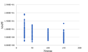
Figure 5
Variation of the mean absolute percentage error (MAPE) considering the number of neurons.

To determine the optimal operational values for the model, we examined the relationship between the number of epochs and the mean squared error (MSE) metric, as depicted in Figure 6. This analysis incorporated findings from previous assessments concerning the number of neurons in the system. To facilitate a clearer interpretation of the data, we arranged the results in ascending order of MSE.

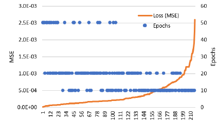
Figure 6
Analysis of mean squared error (MSE) behavior versus number of epochs.

Similar to the analysis in Table 2, notice that when 10 epochs are implemented in the system, there are low performances and high errors. While extending the training to 50 epochs improves outcomes, it significantly increases computational cost. Therefore, using 20 epochs strikes the optimal balance between performance and efficient use of computational resources.

After having performed the analysis of the results, and to obtain the optimum variation of parameters, it was proposed to select the 10 best configurations, taking into account that for efficiency reasons, and as mentioned in Table 2, the tests with 50 epochs will not be taken into account. Table 6 presents various neural network configurations with 150, 100, and 50 neurons in their hidden layers, all maintaining a consistent 20 epochs for training. The ADAM optimizer and the sigmoid activation function were predominantly used across these setups. Among these, test 35 emerged as the most effective option, yielding the best performance.

Table 6
Overall performance results using the MSE as a benchmark

Test	No. Neurons	No. Epochs	Learning rate	Lot size	Optimizer	Output activation	MSE	MAPE	MAE
35	150	20	0,1	1	ADAM	Sigmoid	3,56E-05	3,0250	0,0045
36	150	20	0,1	1	ADAM	Tanh	4,38E-05	3,5740	0,0051
131	50	20	0,1	1	ADAM	Sigmoid	5,59E-05	3,3392	0,0048
29	150	20	0,1	3	ADAM	Sigmoid	5,82E-05	3,3211	0,0050
78	100	20	0,1	3	ADAM	Tanh	6,38E-05	4,0851	0,0048
77	100	20	0,1	3	ADAM	Sigmoid	6,53E-05	3,6244	0,0054
81	100	20	0,1	1	RMSprop	Tanh	6,71E-05	3,3238	0,0045
89	100	20	0,2	3	ADAM	Sigmoid	6,92E-05	2,9174	0,0050
128	50	20	0,1	1	RMSprop	Sigmoid	6,94E-05	3,6845	0,0047
132	50	20	0,1	1	ADAM	Tanh	7,86E-05	6,2786	0,0062

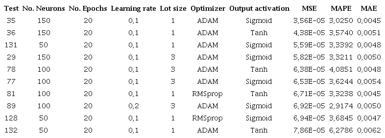
Figure 7 displays four performance graphs of the chosen model. These graphs compare the number of epochs to the mean squared error (MSE), mean absolute error (MAE), and mean absolute percentage error (MAPE), and illustrate the alignment between the predictions of the model and the test data.

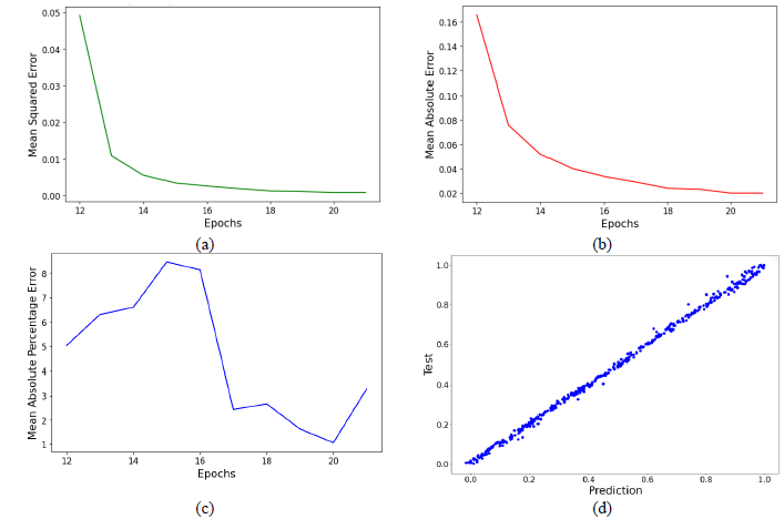
Figure 7
Performance graphs of the selected configuration, showing (a) a decreasing trend in Mean Squared Error over epochs, (b) a decline in Mean Absolute Error with more training iterations, (c) fluctuations in Mean Absolute Percentage Error across epochs, and (d) a scatter plot comparing predicted values against actual test data.

Additionally, Figure 8 illustrates the behavior of the predicted data against the 432 data points used for validation, providing a clear view of the system's operation and its effectiveness.

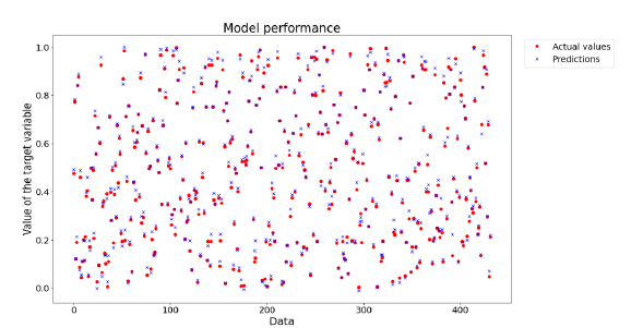
Figure 8
Performance of the selected model. The models presented an input vector that included the surface velocities of each fluid, the internal diameter of the pipe, the velocity of the mixture, and viscosity. Based on performance evaluations, the best model exhibited a mean absolute percentage error of 3.02% and a mean absolute error of 0.0045.

4. Discussion and conclusions

This study demonstrates the potential of Artificial Neural Networks (ANNs) and Long Short-Term Memory (LSTM) networks in predicting the volume fraction of oil in horizontal pipes. Despite the inherent challenges in validating and optimizing these models, their application in the oil and gas industry is promising. Different ANN models using LSTM were defined to calculate the volume fraction of oil and water in horizontal piping through the processing and prediction of data series.

The implementation of an LSTM network showcased the versatility of these models for time series prediction. Furthermore, recent studies have shown that LSTM networks combined with ReLU layers can significantly enhance the accuracy of flow regime prediction in two-phase systems, achieving up to 95.6% accuracy in specific configurations. This is comparable to our model's results, which showed an MSE of 3.5651E-05, underscoring the competitiveness of our LSTM configuration. Another comparative study used GA-BP neural networks and random forest algorithms to predict oil-water flow patterns, achieving up to 93.75% accuracy in some cases. However, our LSTM approach has proven superior in reducing the mean absolute error (MAE) and mean absolute percentage error (MAPE), reinforcing the effectiveness of our network for volume fraction prediction in two-phase flows [11].

The experimental design in this study meticulously assessed the performance of a LSTM neural network in predicting the volume fraction in two-phase flows. Focused on optimizing the predictive accuracy of the model, we varied critical neural network parameters, including the number of neurons, epochs, learning rates, and activation functions. Through 216 distinct tests, each with different configurations, we evaluated the impact of these variations on key metrics such as Mean Squared Error (MSE), Mean Absolute Error (MAE), and Mean Absolute Percentage Error (MAPE). This structured approach enabled the determination of the most effective network configuration, achieving an optimal balance of accuracy and computational efficiency. The selected model incorporated 150 neurons with a ReLU transfer function, two hidden layers, an ADAM optimizer, and an output layer designed for predicting the oil volume fraction.

It is important to note that these models, while accurate, they do not necessarily capture the underlying physics of the problem. However, this limitation highlights the potential for integrating neural networks with traditional Computational Fluid Dynamics (CFD) models. While CFD simulations are known for accurately capturing the physical phenomena in fluid flows, they are computationally expensive, particularly for complex and transient flows. By combining LSTM networks with CFD, it is possible to create hybrid models that leverage the strengths of both approaches maintaining the physical accuracy of CFD while reducing computational costs through neural network approximations. This integration could enhance the predictive capabilities of fluid dynamics models, making them more applicable for realtime and large-scale industrial applications, and offering a promising direction for future research in this field.

Furthermore, while this model was developed specifically for horizontal oil-water flows, its framework can be extended to other multiphase flow scenarios. For instance, with appropriate adjustments, the model could be applied to gas-liquid flows or flows in inclined and vertical pipes. Additionally, the model's adaptability to different geometries and boundary conditions, such as varying pipe diameters or materials, suggests its potential utility in a broad range of industrial applications. Future work could explore these extensions, refining the model to ensure accuracy across diverse conditions.

This research lays the groundwork for future investigations in this field. Continued focus on model validation and optimization could significantly advance predictive capabilities in the oil and gas industry. Future research should aim to improve the robustness of these models and explore their applicability across different operational conditions and pipe configurations.

References

T. Bikmukhametov, J. Jäschke, "First Principles and Machine Learning Virtual Flow Metering: A Literature Review," Journal of Petroleum Science and Engineering, vol. 184, 2020, doi: https://doi.org/10.10167j.petrol.2019.106487

Y. Taitel, A. E. Dukler, "A model for predicting flow regime transitions in horizontal and near horizontal gasliquid flow," AIChE J., vol. 22, no. 1, pp. 47-55, 1976, doi: https://doi.org/10.1002/aic.690220105

D. Barnea, O. Shoham, Y. Taitel, "Flow pattern transition for downward inclined two phase flow; horizontal to vertical," Chem. Eng. Sci., vol. 37, no. 5, pp. 735-740, 1982, doi: https://doi.org/10.1016/0009-2509(82)85033-1

G. A. Valle Tamayo, F. Romero Consuegra, M. E. Cabarcas Simancas, "Predicción de flujo multifásico en sistemas de recolección de crudo: descripción de requerimientos," Rev. Fuentes el Reventón Energético, vol. 15, no. 1, pp. 87-99, 2017, doi: https://doi.org/10.18273/revfue.v15n1-2017008

O. S. Osundare, G. Falcone, L. Lao, A. Elliott, "Liquid-liquid flow pattern prediction using relevant dimensionless parameter groups," Energies, vol. 13, no. 17, 2020, doi: https://doi.org/10.3390/en13174355

C. R. K. García, J. García, G. Montoya, M. T. Valecillos, "Determinación de altura de fase y Hold Up para flujo bifásico líquido-líquido en tuberías horizontales por medio de procesamiento de imágenes," in VIII Congreso anual de ingeniería ASME, Caracas, Venezuela, 2009, pp. 1-10.

N. Varotsis, "Prediction of gas phase volumetric variations in diphasic reservoir oils," J. Can. Pet. Technol., vol. 36, no. 8, pp. 56-60, 1997, doi: https://doi.org/10.2118/97-08-05

M. R. Malayeri, H. Müller-Steinhagen, J. M. Smith, "Neural network analysis of void fraction in air/water two-phase flows at elevated temperatures," Chem. Eng. Process. Process Intensif., vol. 42, no. 8-9, pp. 587-597, 2003, doi: https://doi.org/10.1016/S0255-2701(02)00208-8

M. Abdelhafidh, M. Fourati, L. C. Fourati, A. Abidi, "Remote water pipeline monitoring system IoT-based architecture for new industrial era 4.0," Proc. IEEE/ACS Int. Conf. Comput. Syst. Appl. AICCSA, vol. 2017-Octob, pp. 1184-1191, 2018, doi: https://doi.org/10.1109/AICCSA.2017.158

V. Slany, A. Lucansky, P. Koudelka, J. Marecek, E. Krcálová, R. Martínek, "An integrated iot architecture for smart metering using next generation sensor for water management based on lorawan technology: A pilot study," Sensors, vol. 20, no. 17, pp. 1-23, 2020, doi: https://doi.org/10.3390/s20174712

C. M. Ruiz-Díaz, B. Quispe-Suarez, O. A. González-Estrada, "Two-phase oil and water flow pattern identification in vertical pipes applying long short-term memory networks," Emergent Mater., pp. 113, 2024, doi: https://doi.org/10.1007/s42247-024-00631-2

A. Ibrahim, B. Hewakandamby, Z. Yang, B. Azzopardi, "Effect of liquid viscosity on two-phase flow development in a vertical large diameter pipe," Am. Soc. Mech. Eng. Fluids Eng. Div. FEDSM, vol. 3, pp. 1-10, 2018, doi: https://doi.org/10.1115/FEDSM2018-83466

K. R. Sai, P. J. Nayak, K. V. A. Kumar, A. D. Dutta, "Oil Spill Management System Based on Internet of Things," Proc. 2020IEEE-HYDCONInt. Conf. Eng. 4^thInd. Revolution, HYDCON 2020, 2020, doi: https://doi.org/10.1109/HYDCON48903.2020.9242823

C. Gomez, D. Ruiz, M. Cely, "Specialist system in flow pattern identification using artificial neural Networks," J. Appl. Eng. Sci., vol. 21, no. 2, pp. 285-299, Jan. 2023, doi: https://doi.org/10.5937/jaes0-40309

C. Ruiz-Diaz, M. M. Hernández-Cely, O. A. González-Estrada, "Modelo predictivo para el cálculo de la fracción volumétrica de un flujo bifásico agua- aceite en la horizontal utilizando una red neuronal artificial," Rev. UIS Ing., vol. 21, no. 2, pp. 155-164, 2022, doi: https://doi.org/10.18273/revuin.v21n2-2022013

V. Ganeshmoorthy, M. Muthukannan, M. Thirugnanasambandam, "Comparison of Linear Regression and ANN of Fish Oil Biodiesel Properties Prediction," J. Phys. Conf. Ser., vol. 1276, no. 1, 2019, doi: https://doi.org/10.1088/1742-6596/1276/1/012074

S. Chaki, A. K. Verma, A. Routray, W. K. Mohanty, M. Jenamani, "Well tops guided prediction of reservoir properties using modular neural network concept: A case study from western onshore, India," J. Pet. Sci. Eng., vol. 123, pp. 155-163, 2014, doi: https://doi.org/10.1016/j.petrol.2014.06.019

C. M. Ruiz-Diaz, M. M. Hernández-Cely, O. A. González-Estrada, "A Predictive Model for the Identification of the Volume Fraction in Two-Phase Flow," Cienc. en Desarro., vol. 12, no. 2, pp. 49-55, 2021.

Q. Cao, R. Banerjee, S. Gupta, J. Li, W. Zhou, B. Jeyachandra, "Data driven production forecasting using machine learning," SPE Argentina Exploration and Production of Unconventional Resources Symposium, 2016. doi: https://doi.org/10.2118/180984-MS

G. Luo, Y. Tian, M. Bychina, C. Ehlig-Economides, "Production optimization using machine learning in bakken shale," SPE/AAPG/SEG Unconv. Resour. Technol. Conf.2018, URTC2018, no. 2011, 2018, doi: https://doi.org/10.15530/urtec-2018-2902505

A. U. Osarogiagbon, F. Khan, R. Venkatesan, P. Gillard, "Review and analysis of supervised machine learning algorithms for hazardous events in drilling operations," Process Saf. Environ. Prot., vol. 147, pp. 367-384, 2021, doi: https://doi.org/10.1016/j.psep.2020.09.038

Z. Zhong, T. R. Carr, X. Wu, G. Wang, "Application of a convolutional neural network in permeability prediction: A case study in the Jacksonburg-Stringtown oil field, West Virginia, USA," Geophysics, vol. 84, no. 6, pp. B363-B373, 2019, doi: https://doi.org/10.1190/geo2018-0588.1

C. M. Salgado, R. S. F. Dam, W. L. Salgado, M. C. Santos, and R. Schirru, "Development of a deep rectifier neural network for fluid volume fraction prediction in multiphase flows by gamma-ray densitometry," Radiat. Phys. Chem., vol. 189, no. July, p. 109708, 2021, doi: https://doi.org/10.1016/j.radphyschem.2021.109708

P. Temirchev et al., "Deep neural networks predicting oil movement in a development unit," J. Pet. Sci. Eng., vol. 184, no. August 2019, p. 106513, 2020, doi: https://doi.org/10.1016/j.petrol.2019.106513

D. Biswas, "Adapting shallow and deep learning algorithms to examine production performance - Data analytics and forecasting," Soc. Pet. Eng. - SPE/IATMI Asia Pacific Oil Gas Conf. Exhib. 2019, APOG 2019, 2019, doi: https://doi.org/10.2118/196404-ms

S. Madasu, K. P. Rangarajan, "Deep recurrent neural network DrNN model for real-time step-down analysis," Soc. Pet. Eng. - SPE Reserv. Characterisation Simul. Conf. Exhib. 2019, RCSC 2019, 2019, doi: https://doi.org/10.2118/196621-ms

H. Li, S. Misra, J. He, "Neural network modeling of in situ fluid-filled pore size distributions in subsurface shale reservoirs under data constraints," Neural Comput. Appl., vol. 32, no. 8, pp. 3873-3885, Apr. 2020, doi: https://doi.org/10.1007/s00521-019-04124-w

A. Sagheer, M. Kotb, "Time series forecasting of petroleum production using deep LSTM recurrent networks," Neurocomputing, vol. 323, pp. 203-213, 2019, doi: https://doi.org/10.1016Zj.neucom.2018.09.082

H. D. Pasinato, N. F. M. Reh, "Modeling Turbulent Flows with LSTM Neural Network," arXiv.org, Jul. 2023, doi: https://doi.org/10.48550/arxiv.2307.13784

R. Vinuesa, S. L. Brunton, "Enhancing computational fluid dynamics with machine learning," Nat. Comput. Sci., vol. 2, no. 6, pp. 358-366, Jun. 2022, doi: https://doi.org/10.1038/s43588-022-00264-7

P. A. Costa Rocha, S. J. Johnston, V. Oliveira Santos, A. A. Aliabadi, J. V. G. Thé, B. Gharabaghi, "Deep Neural Network Modeling for CFD Simulations: Benchmarking the Fourier Neural Operator on the Lid-Driven Cavity Case," Appl. Sci., vol. 13, no. 5, p. 3165, 2023, doi: https://doi.org/10.3390/app13053165

A. F. Casas-Pulido, M. M. Hernández-Cely, O. M. Rodríguez-Hernández, "Análisis experimental de flujo líquido-líquido en un tubo horizontal usando redes neuronales artificiales," Rev. UIS Ing., vol. 22, no. 1, pp. 49-56, Jan. 2023, doi: https://doi.org/10.18273/revuin.v22n1-2023005

C. M. Ruiz-Díaz , E. E. Perilla-Plata, O. A. González-Estrada, "Two-Phase Flow Pattern Identification in Vertical Pipes Using Transformer Neural Networks," Inventions, vol. 9, no. 1, p. 15, Jan. 2024, doi: https://doi.org/10.3390/inventions9010015

J. Shi, L. Lao, H. Yeung, "Water-lubricated transport of high-viscosity oil in horizontal pipes: The water holdup and pressure gradient," Int. J. Multiph. Flow, vol. 96, no. July, pp. 70-85, Nov. 2017, doi: https://doi.org/10.1016/j.ijmultiphaseflow.2017.07.005

P. Abduvayt, R. Manabe, T. Watanabe, N. Arihara, "Analisis of Oil-Water Flow Tests in Horizontal, Hilly-Terrain, and Vertical Pipes," in Proceedings of SPE Annual Technical Conference and Exhibition, Sep. 2004, pp. 1335-1347. doi: https://doi.org/10.2523/90096-MS

J. Cai, C. Li, X. Tang, F. Ayello, S. Richter, S. Nesic, "Experimental study of water wetting in oil-water two phase flow-Horizontal flow of model oil," Chem. Eng. Sci., vol. 73, pp. 334-344, May 2012, doi: https://doi.org/10.1016/j.ces.2012.01.014

A. Al-Sarkhi, E. Pereyra, I. Mantilla, C. Avila, "Dimensionless oil-water stratified to non-stratified flow pattern transition," J. Pet. Sci. Eng., vol. 151, no. September 2016, pp. 284-291, 2017, doi: https://doi.org/10.1016/j.petrol.2017.01.016

J. Shi, L. Lao, H. Yeung, "Water-lubricated transport of high-viscosity oil in horizontal pipes: The water holdup and pressure gradient," Int. J. Multiph. Flow, vol. 96, pp. 70-85, 2017, doi: https://doi.org/10.1016/j.ijmultiphaseflow.2017.07.005

T. Al-Wahaibi et al., "Experimental investigation on flow patterns and pressure gradient through two pipe diameters in horizontal oil-water flows," J. Pet. Sci. Eng., vol. 122, pp. 266-273, 2014, doi: https://doi.org/10.1016/j.petrol.2014.07.019

A. Dasari, A. B. Desamala, A. K. Dasmahapatra, T. K. Mandal, "Experimental studies and probabilistic neural network prediction on flow pattern of viscous oil-water flow through a circular horizontal pipe," Ind. Eng. Chem. Res., vol. 52, no. 23, pp. 7975-7985, 2013, doi: https://doi.org/10.1021/ie301430m

R. Ibarra, I. Zadrazil, C. N. Markides, O. K. Matar, "Towards a universal dimensionless map of flow regime transitions in horizontal liquid-liquid flows," in 11thInternational Conference on Heat Transfer, Fluid Mechanics and Thermodynamics, 2015, no. July, pp. 2023.

M. Nädler, D. Mewes, "Flow induced emulsification in the flow of two immiscible liquids in horizontal pipes," Int. J. Multiph. Flow, vol. 23, no. 1, pp. 55-68, 1997, doi: https://doi.org/10.1016/S0301-9322(96)00055-9

O. M. H. Rodriguez, R. V. A. Oliemans, "Experimental study on oil-water flow in horizontal and slightly inclined pipes," Int. J. Multiph. Flow, vol. 32, no. 3, pp. 323-343, 2006, doi: https://doi.org/10.1016/j.ijmultiphaseflow.2005.11.001

Z. Qiao, Z. Wang, C. Zhang, S. Yuan, Y. Zhu, J. Wang, "PVAm-PIP/PS composite membrane with high performance for CO2/N2 separation," AIChE J., vol. 59, no. 4, pp. 215-228, 2012, doi: https://doi.org/10.1002/aic

A. Wegmann, P. Rudolf von Rohr, "Two phase liquid-liquid flows in pipes of small diameters," Int. J. Multiph. Flow, vol. 32, no. 8, pp. 1017-1028, 2006, doi: https://doi.org/10.1016/j.ijmultiphaseflow.2006.04.001

W. McKinney, "Data Structures for Statistical Computing in Python," Proceedings of the 9th Python in Science Conference, 2010, pp. 56-61, doi: https://doi.org/10.25080/majora-92bf1922-00a

S. Hochreiter, J. Schmidhuber, "Long Short-Term Memory," Neural Comput., vol. 9, no. 8, pp. 1735-1780, Nov. 1997, doi: https://doi.org/10.1162/neco.1997.9.8.1735

K. Greff, R. K. Srivastava, J. Koutnik, B. R. Steunebrink, J. Schmidhuber, "LSTM: A Search Space Odyssey," IEEE Trans. Neural Networks Learn. Syst., vol. 28, no. 10, pp. 2222-2232, Oct. 2017, doi: https://doi.org/10.1109/TNNLS.2016.2582924

How to cite:

Funding acquisition

Autor Contributions

Institutional Review Board Statement

Informed Consent Statement

Author notes

^a Emails: cahss77@hotmail.com^balejandro.cv0414@gmail.com^cagonzale@uis.edu.co

Conflict of interest declaration