
This work is licensed under Creative Commons Attribution 4.0 International.
Received: 10 May 2016
Accepted: 29 May 2017
DOI: https://doi.org/10.1016/j.rausp.2017.08.003
Abstract: The purpose of this paper is to investigate the volatility persistence and the inventory effect in grain futures markets during the period of 1959–2014. The innovative nature of this study lies in the evaluation of rolling estimates, using a recursive univariate TARCH(1,1)-in-mean volatility model. The daily evolution of volatility persistence and the inventory effect on corn and soybean futures contracts is analyzed using a rolling window of 1008 observations over four years. In general, the results suggest that the conditional volatility in both markets is highly persistent. There is also evidence of inventory, time-to-maturity, and seasonality effects on the volatility dynamics of corn and soybeans. In addition, the findings point to a lower short-run volatility persistence in recent years, which caused a slight decrease in long-run volatility persistence and the half-life period in both markets.
Keywords: Price volatility, Volatility persistence, Inventory effect, Grain futures markets.
Resumo: Neste artigo, os autores procuraram investigar a persistência da volatilidade e inventory effect nos mercados futuros de grãos no período entre 1959 e 2014. A inovação do estudo consistiu na aplicação de um modelo de volatilidade recursivo TARCH(1,1) com rolagem das estimativas a partir de uma janela de tempo de quatro anos. Os resultados apontaram para uma alta persistência da volatilidade condicional nos mercados de milho e soja. Além disso, observou-se a presença dos efeitos sazonalidade, inventory e time-to-maturity na dinâmica de volatilidade dos preços de ambos mercados. Verificou-se ainda uma queda na persistência de curto-prazo no período recente, o que levou a uma diminuição da persistência de longo-prazo e da meia-vida nos mercados em estudo.
Palavras-chave: Volatilidade, Persistência da volatilidade, Inventory effect, Mercado futuro de grãos.
Resumen: El objetivo en este estudio es investigar la persistencia de la volatilidad y el efecto de inventario en los mercados de futuros de granos en el período de 1959 a 2014. La innovación del trabajo consiste en la aplicación de un modelo de volatilidad recursivo TARCH(1,1) por estimación, en un período de cuatro años. Los resultados indican una alta persistencia de la volatilidad condicional en el mercado de maíz y soja. Además, hay evidencia de efectos de inventario, tiempo hasta la expiración y estacionalidad en la dinámica de la volatilidad de los precios de ambos mercados. También se ha verificado una baja persistencia de la volatilidad a corto plazo en los últimos años, lo que ha causado una caída de la persistencia de la volatilidad a largo plazo.
Palabras clave: Volatilidad, Persistencia de la volatilidad, Efecto de inventario, Mercado futuro de granos.
INTRODUCTION
The analysis of price volatility in agricultural markets plays an important role in the decision-making process. Price variation influences decision-making in the case of production, marketing, and risk management in agriculture. High price fluctuations affect producer's profitability, even when production is very efficient. These events also affect policy makers, especially in developing countries, since price and volatility levels impact food security, balance of trade, inflation rate, tax revenue, employment, GDP, and business cycles. Additionally, in financial markets, price oscillations are relevant in portfolio allocation and derivatives pricing (Ghoshray, 2013; Naylor & Falcon, 2010).
During the 2000s, many agricultural commodities experienced a sharp and rapid rise in price. While over the second half of the 1970s and 1990s, in particular in the 1980s, the inflation-adjusted World Bank agriculture index decreased 58%, a sharp price spike of around 40% occurred during 2005–2008. Agricultural commodities, such as corn, wheat, and soybeans exhibited a price increase of more than 60% over this period.
Previous studies have investigated the factors underlying this scenario. Several explanations were given, such as an increasing demand for biofuel from grains and oilseeds, rising oil prices, a growth in demand for commodities (especially in the BRICS countries – Brazil, Russia, India, China, and South Africa), a reduction in subsidies for European farmers, adverse weather conditions, low inventory levels, depreciation of the U.S. dollar, and an increase in speculative transactions in commodities futures markets (Gilbert, 2010; Headey & Fan, 2008; Sumner, 2009).
Recent studies have explored the price fluctuations of agricultural commodities in order to verify the existence of volatility breaks in the first decade of the 2000s (Calvo-Gonzalez, Shankar, & Trezzi, 2010; Gilbert & Morgan, 2010; Huchet-Bourdon, 2011; Sumner, 2009; Vivian & Wohar, 2012). In general, no clear evidence was found to support the idea that the recent price variability was unparalleled. However, two important issues have received relatively little attention, namely the persistence of price volatility and the leverage effect (also known as the "inventory effect", in the case of commodities). Even if agricultural markets are not experiencing unprecedented levels of volatility, it is still crucial to understand how long it takes volatility to revert to its previous level after a shock. In addition, it is important to verify the asymmetry in the volatility process. In agricultural markets, in contrast to equity markets, positive price shocks ("bad news") tend to have a larger impact on conditional variance than negative price shocks ("good news"). This phenomenon is known as the inventory effect (Carpantier, 2010) and can be explained by the storage model.[1] Volatility persistence and inventory effects affect agricultural producers', buyers', and traders' exposure to risk, thus influencing risk management operations (Carpantier & Samkharadze, 2013). More broadly, these issues are relevant for countries that rely heavily on exports and imports of agricultural commodities, as well as to evaluate inflationary processes and formulate price stabilization programs (Ghoshray, 2013; Vivian & Wohar, 2012).
This paper explores the volatility persistence and inventory effect on grain futures markets over the last decades. The research uses daily futures prices of two commodities (corn and soybeans). A recursive univariate TARCH(1,1)-in-mean volatility model is applied to compute the daily evolution of the volatility persistence and the inventory effect in terms of rolling estimates. Thus, the study investigates whether there have been changes in these two measures over time and their implications for agricultural markets. The study also analyzes other determinants of agricultural commodity volatility in model specification, such as seasonality and time-to-maturity.
Previous studies
Several empirical studies have employed different approaches to investigate the volatility dynamics in agricultural markets. These studies can be categorized into five main groups. The first one evaluated and compared price and volatility evolution between agricultural commodities and manufactured goods. Prebisch (1950) and Singer (1950) began this analysis and, more recently, other research has focused on price volatility, such as Jacks, O'Rourke, and Williamson (2011), Arezki, Hadri, Loungani, and Rao (2014) and Arezki, Lederman, and Zhao (2014). The second group of studies analyzed the impact of commodity price volatility on income and welfare in developing countries (Bellemare, Barrett, & Just, 2013; Blattman, Hwang, & Williamson, 2007; Naylor & Falcon, 2010; Rapsomanikis & Sarris, 2008).
A third group of studies compared commodity price volatility between the first decade of the 21st century and the previous decades of the 20th century. In general, the results showed that price variability over 2006–2010 was not higher than the volatility observed in 1970 (Gilbert & Morgan, 2010; Huchet-Bourdon, 2011). Calvo-Gonzalez et al. (2010) highlighted three periods of relevant volatility breaks – during the two world wars and during the time when the Bretton Woods system collapsed. Despite the fact that the commodity volatility level during the 2000s was not unparalleled, relevant spikes were observed from 2005 to 2008. Consequently, a number of works have evaluated the causes of the rising volatility, enumerating factors such as the fast expansion of biofuel production, increasing oil prices, depreciation of the U. S. dollar, lower level of inventories and the "financialization" of commodity markets (Arezki, Loungani, Ploeg, & Venables, 2014; Balcombe, 2009; Beckmann & Czudaj, 2014; Du, Yu, & Hayes, 2011; Mensi, Beljid, Boubaker, & Managi, 2013; Nazlioglu, Erdem, & Soytas, 2013; Power & Robinson, 2013; Serra, 2011; Wright, 2011).
In addition, a fourth group of studies analyzed the determinants of agricultural commodity price volatility. Seasonality, time-to-maturity,[2] inventory level, volatility persistence, day-of-the-week, futures market trading volume, speculative activity, loan rate level, price level, among others, were analyzed in order to verify their influence on agricultural commodity price fluctuation. Table 1 present a summary of this literature and the following paragraphs address the recent studies.
Summary of literature reviews regarding the determinants of agricultural commodity volatility

Y, yes; N, no; NS, not studied.
A number of works have identified seasonality and time-to-maturity as important determinants of agricultural volatility. Kalev and Duong (2008) and Duong and Kalev (2008), using intraday data, verified the maturity effect in agricultural futures markets. In addition, Karali and Thurman (2010) identified the presence of seasonality and maturity effects in corn, soybean, wheat, and oats markets between 1986 and 2007. Karali et al. (2010) showed that the volatility of corn, soybean, and oats futures prices was affected by time-to-maturity, inventories, and progress of the crop (with, in general, a higher price fluctuation before the beginning of the harvest). Verma and Kumar (2010) and Gupta and Rajib (2012) also contributed to this debate, examining the time-to-maturity effect in Indian futures markets. On one hand, Verma and Kumar (2010) found evidence of a maturity effect in wheat and pepper futures markets. On the other hand, Gupta and Rajib (2012), focusing the analysis on eight commodities futures markets (including wheat futures contract), indicated that the futures contract trading volume has a higher effect on the volatility than time-to-maturity. He, Yang, Xie, and Han (2014) confirmed the importance of the volume effect on price volatility, by studying six commodities futures markets in China.
Many studies have also indicated the inventory effect as a relevant factor that influences agricultural price variability. Carpantier (2010) analyzed 15 commodity price series over 1994–2009 and found that there was an inventory effect in coffee, soybean, and wheat markets. A similar analysis was carried out by Carpantier and Dufays (2012), analyzing 16 commodities from 1994 to 2011. All of the estimated asymmetric coefficients for agricultural markets (corn, cotton, soybean, sugar, wheat, and coffee) were negative, however, only in the cases of sugar and coffee were the parameters statistically different from zero. Stigler and Prakash (2011) verified two distinct levels of unconditional volatility in the wheat market, where one regime oscillated between 20 and 36 times higher than the other regime. The authors showed that the higher volatility regime emerged when the United States Department of Agriculture (USDA) forecasts pointed to a low inventory level (bad news on stocks-to-disappearance). Conversely, when the USDA inventory forecasts indicated no market tightness (positive news on stocks-to-disappearance), there was no apparent relationship between wheat prices and inventory level.
Finally, the volatility persistence of agricultural commodities was evaluated by a fifth group of studies. Balcombe (2009) investigated the factors that drove the volatility of 19 agricultural commodities over the last decades. He not only found evidence of a high volatility persistence in all price series but also that oil volatility, inventory levels, and yields influence price variability. Vivian and Wohar (2012) indicated, in general, a high volatility persistence considering 28 commodities (grains, animals, metals, and energy) over the years 1985–2010. Ghoshray (2013) also examined the volatility persistence of 24 commodity prices series during the 1900–2008 period. The results suggested that the volatility persistence varies significantly over time and between different products. Using a spline-GARCH model, Karali and Power (2013) found that the volatility persistence is lower than the one estimated from standard GARCH models in the agricultural, energy, and metal futures markets. In addition, Khan (2014) and Dawson (2015) indicated a high volatility persistence in cotton and wheat futures market, respectively. Khan (2014) also verified that cotton volatility was impacted by stocks-to-use ratio, price level, and futures market concentration.
Overall, previous studies have found that the volatility increased during the 2000s financial crisis, but that it was not higher than the price variability verified in other decades. In addition, the researches, in general, stated not only the presence of volatility persistence, but also the evidence of inventory, maturity, and seasonality effects on agricultural price fluctuations. The present study contributed to this debate by exploring the evolution of the inventory effect and volatility persistence rolling estimates using a recursive univariate TARCH(1,1)-in-mean volatility model. The work also evaluates the influence of seasonality and time-to-maturity. In the following section, the methodology used to achieve these goals is described.
RESEARCH METHOD
According to the literature, futures prices returns of agricultural commodities (Eq. (1)) do not generally follow a normal distribution, given the presence of nonzero skewness and kurtosis greater than three (Isengildina, Irwin, & Good, 2006; Karali, 2012). Thus, GARCH models are more suitable for such series (Hováth & Sapov, 2016; Pockhilchuck & Savel'ev, 2016; Watkins & Mcaleer, 2008). In addition, taking into account that markets react asymmetrically to good news and bad news, a Threshold Autoregressive Conditional Heteroskedasticity (TARCH) model is chosen to capture the volatility process (Zakoian, 1994). Eqs. (2) and (3) describe the TARCH(1,1)-in-mean model:
Rt=ln()×100 (1)
Rt=δ0+δ1Rt−1+δ2ht+εt (2)
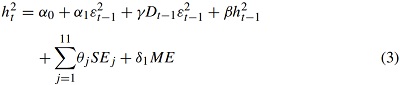
In Eq. (1), Rt represents the daily percentage of close-to-close futures prices returns, which is obtained by comparing the closing price of the nearest-to-maturity futures contract on day t (Pt) to the closing prices on day t − 1 (Pt−1). In (2), the mean equation, δ0 is a constant, Rt−1 lagged daily return to account for autocorrelation in futures returns (Isengildina et al., 2006; Karali, 2012), ht the conditional standard deviation to capture the effects of the volatility on the mean term, and ɛt the error term such that ɛt|Ωt−1 ∼ N(0, h2t), where Ωt−1 represents the information available in t − 1. Finally, Eq. (3) represents the conditional variance h2t≡VAR(Rt|Ωt−1). The lagged squared residual in the mean equation, εt−12, is used to represent volatility shocks from the previous day. Additionally, a binary variable Dt−1 is included to explore asymmetric effects, such that Dt−1 equals 1 when ɛt−1 is negative and 0 when ɛt−1 is positive. Thus, the impact of positive volatility shocks is given by α1, while the impact of negative volatility shocks is given by (α1 + γ). A statistically significant estimate for γ implies the existence of asymmetry in volatility. A negative γ provides evidence of the inventory effect, i.e. positive volatility shocks in t − 1 increase conditional volatility in t proportionally more than negative volatility shocks. Another variable in Eq. (3) is the lagged conditional variance, ht−12. The volatility persistence in a TARCH model is given by (α1 + γ/2 + β). As this sum tends to one, a given shock in return takes longer to dissipate.
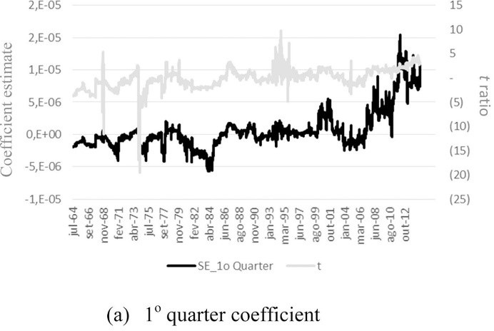
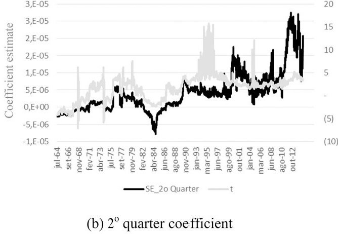
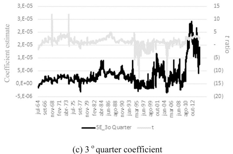
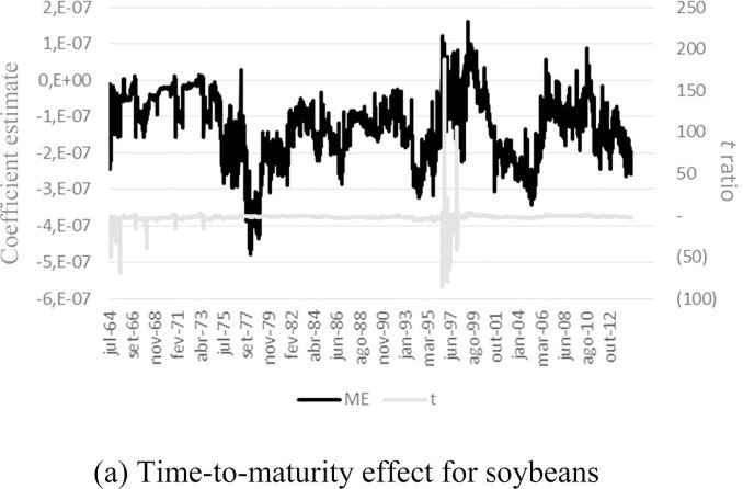
Two types of external effects are incorporated into the variance equation: seasonality and time-to-maturity. The seasonality effect is included using three variables SEj for quarters of the year: SE1 equals 1 for January, February, and March, and 0 otherwise; SE2 equals 1 for April, May, and June, and 0 otherwise; SE3 equals 1 for July, August, and September, and 0 otherwise. The maturity effect is expressed by the variable ME and should be negatively related to the commodity price volatility, since price variability tends to increase as the maturity date approaches.
The model is estimated recursively by the maximum likelihood method, using a rolling window of 1008 observations (4 years). This method makes it possible to analyze how volatility parameter estimates change over time. In this way, the daily evolution of the volatility persistence and the inventory effect are analyzed in terms of the rolling parameters estimate. Note that several different structures were estimated for the model using maximum likelihood, and the final specification was selected in terms of parsimony by the Schwarz Information Criteria (BIC). Since the aim of the paper is to evaluate the volatility pattern over time by means of recursive parameter estimates, a model with many parameters compromises the interpretability and requires higher computational costs, which can result in unstable time series of estimated parameters. The BIC indicated that the structure in Eqs. (1)–(3) is able to capture volatility dynamics accurately with relatively few parameters.
Data
The data set consists of futures prices of corn and soybeans. Futures prices are daily closing quotes for nearby contracts from the Chicago Mercantile Exchange Group (CME) between July 1959 and December 2014. Fig. 1 presents the evolution of daily futures prices and returns for corn and soybeans.
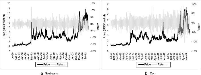
Fig. 1
Daily futures prices and percentage daily returns for soybeans and corn (July 1959–December 2014).
Descriptive statistics for corn and soybean returns are given in Table 2. Mean returns (Rt) of corn are not statistically distinguishable from zero. Mean absolute returns (|Rt|) are in the 0.96–1.02% range and are also statistically distinguishable from zero. A similar volatility in the soybean and corn futures market can be observed. Soybean returns have a daily standard deviation of 1.46% per day (23.15% per year), while corn shows 1.39% per day (22.01% per year). In addition, regarding the return series, there is no evidence of skewness, however, the distributions of absolute returns appear to be positively skewed. There is also evidence of excess kurtosis for both series. Finally, Jarque–Bera tests suggest nonnormality in all series, supporting findings given by previous studies (Isengildina et al., 2006; Karali, 2012).
Descriptive statistics of daily returns percentage and absolute percentage daily returns for soybeans and corn July 1959December 2014
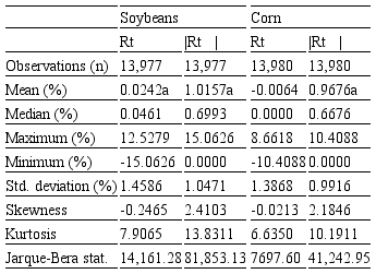
aStatistically distinguishable from zero at 10%.
RESULTS
Volatility series for soybeans and corn are obtained through the estimation of the TARCH model (Eq. (3)). Results indicate the existence of volatility clusters for corn and soybean returns. In both markets, annual volatility generally ranges between 10% and 50%. In addition, the three most relevant breaks in price volatility common to corn and soybeans occurred at the end of Bretton Woods system (1973), the largest production shortfall in the U.S. grain markets in 1988, and during the subprime crisis in 2008. During these periods, the volatility in grain markets exceeded 60% a.a (Fig. 2).
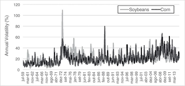
Fig. 2
Estimated conditional standard deviation for soybean and corn returns (July 1959–December 2014).
Table 3 presents the results of the estimated TARCH model for soybean futures returns. Estimated coefficients for the soybean model between July 1959 and December 2014 are reported in column I. The model was also estimated over four different periods, according to grain price evolution: 1959–1972 (column II), 1973–1988 (column III), 1989–2004 (column IV), and 2005–2014 (column V). In general, results suggest that conditional volatility is highly persistent (i.e. volatility shocks would take several days to decay) in all periods. The half-life period[3] of futures price responses to a random shock is 374 days, indicating a slow adjustment process. Results also suggest a fall in half-life period during the four split periods, exhibiting 154, 93, 64 and 47 days, respectively.
TARCH model estimates for soybean returns
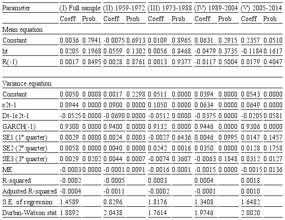
Further, there is evidence of an asymmetric effect of volatility shocks in the soybean market (Table 3). Estimated coefficients of the term Dt−1ε2t−1 are negative, which means that positive shocks appear to have a greater effect on the conditional variance than negative price shocks. In addition, there is also evidence of the time-to-maturity effect, since the ME estimated coefficient is negative and statistically distinguishable from zero in all periods. Thus, when a soybean futures contract approaches its expiration, volatility increases. With respect to the seasonality effect, in general, results indicate higher volatility in the second quarter, during the planting period in the U.S.
Table 4 shows the results of the estimated TARCH model for corn futures returns. Again, estimated coefficients for the model, considering the complete sample, are reported in column I, and for the model considering different periods in columns II (1959–72), III (1973–88), IV (1989–2004), and V (2005–2014). Estimated coefficients for ε2t−1 and h2.−1 are statistically distinguishable from zero during all periods, implying that previous shocks and the volatility forecast impact the conditional variance in corn.
TARCH model estimates for corn returns
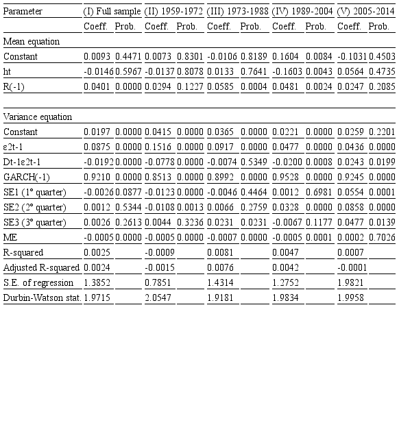
In addition, in the variance equation, the model shows high volatility persistence. For the years 1959–2014, the half-life period is 630 days, indicating a very slow adjustment process. Regarding the split periods, the models show a half-life of 19 days for 1959–1972, 54 days for 1973–1988, 73 days for 1989–2004, and 35 days for 2005–2014.
There is also evidence of inventory and time-to-maturity effects in all periods (except during 2005–2014). Furthermore, results suggest higher volatility in the second quarter compared to the rest of the year.
Overall, results suggest changes in the estimated parameters. In both markets, we can verify a slightly lower short-run persistence (ε2t−1) and a slightly higher asymmetric effect (D.−1ε2t−1), particularly between 2005 and 2014. Furthermore, there is evidence of maturity and seasonality effects. Rolling coefficient estimates, which are discussed as follows, provide a more comprehensive analysis of these issues and shed more light on the analysis.
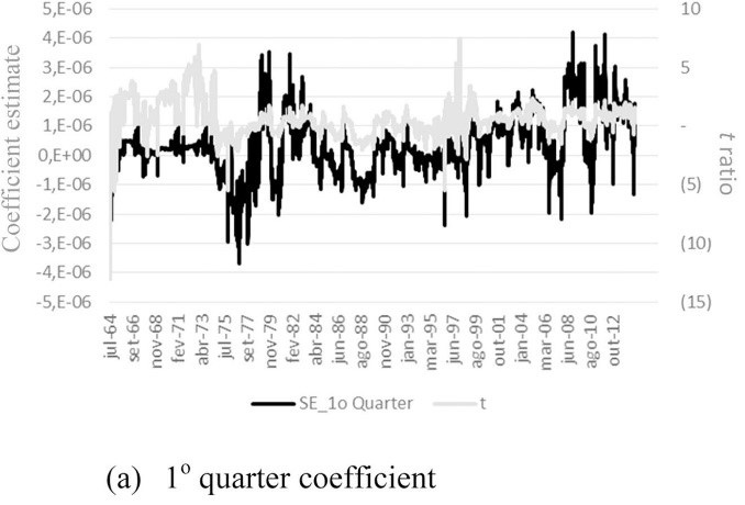
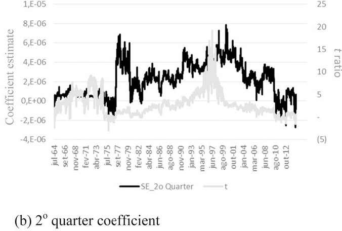
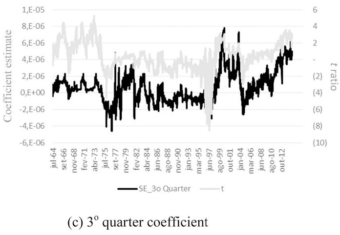
Fig. 3 shows the evolution of rolling .1, . and . coefficient estimates with a rolling window of 1008 observations for corn and soybeans and their corresponding .-ratios from July 1963 to December 2014. In general, rolling . coefficient estimates for corn and soybean models are in the 0.8–1.0 range and are statistically distinguishable from zero, which indicates greater long-run shock persistence. For corn, . coefficient estimates present lower levels and higher instability than the respective soybean parameter (Table 5).
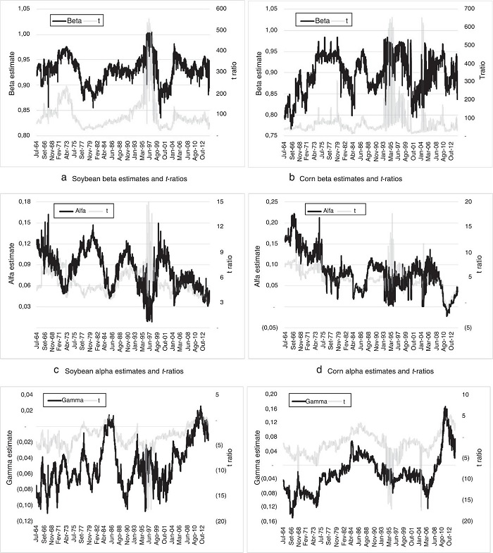
Fig. 3
Rolling coefficient estimates for soybeans and corn.
Descriptive statistics for rolling α 1 β and γ coefficient estimates and halflife period.
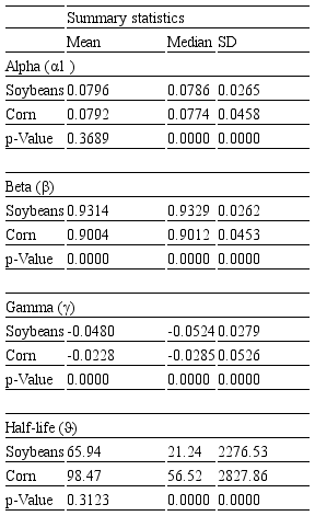
With respect to rolling .1 coefficient estimates, which indicate short-run persistence, the values oscillated between 0–0.15 for soybean and 0–0.20 for corn (Fig. 3). In addition, rolling . coefficient estimates for corn and soybeans seemed to present similar levels, along with higher variability for corn (Table 5). Finally, rolling . coefficient estimates for soybeans (corn) vary between −0.10 and 0.02 (−0.15 and 0.15). The . estimates from the corn model also show higher values and greater variability than the estimates from the soybean model. In general, since the coefficient is usually negative, there is evidence of an inventory effect.
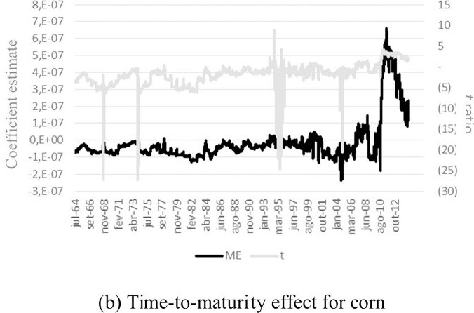
Furthermore, Appendices A–C present the rolling coefficient estimates for seasonality and time-to-maturity effects for the soybean and corn markets. Results point to the existence of greater volatility during the planting period and before the harvest in the U.S. (second and third quarters). The evolution of time-to-maturity coefficient indicates higher futures price variability when the futures contract approaches its expiration for both markets.
Table 6 shows the descriptive statistics for rolling .1, . and . coefficient estimates for each separate period. The findings confirm previous results related to lower . estimates over the last two periods, resulting in a decrease in the importance of short-run volatility persistence in soybean and corn markets. Consequently, it can be largely verified that the long-run persistence (.1 + ./2 + .) and half-life period tend to be lower in the recent period, especially during 2005–2014, despite increasing values for ..
Descriptive statistics for rolling α β and γ coefficient estimates and halflife period during 19591972 19731988 19892004 and 20052014.
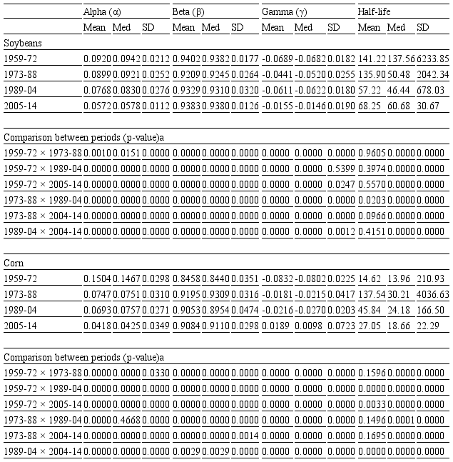
ap-Value for the hypothesis test that the population statistics are equal.
CONCLUSIONS
Agricultural markets are largely characterized by high price volatility, due to the low price elasticity of supply. This characteristic highlights the risk of this activity, which represents a susceptibility factor for primary producing countries. During the first decade of the 2000s, major agricultural commodities experienced a sharp and rapid rise in price and volatility, thus stimulating discussions and research in order to understand the reasons that led to such a scenario. With the increase in biofuel production from grains and oilseeds and restriction of acreage growth due to environmental issues, the pressure on agricultural areas will intensify, which may be reflected in increasing food prices.
Studies that investigate price volatility patterns in agricultural markets have significant importance, since they can help to improve decision-making processes related to production, risk management and marketing. In addition, policy makers can also benefit from these studies as they analyze the impacts of energy policies on agricultural price and food security. This paper contributes to the recent debate about volatility in agricultural markets by focusing the analysis on grain volatility persistence and the inventory effect. Using a conditional volatility model to generate rolling estimates, this work provides evidence on the evolution of volatility, its persistence and the inventory effect over the last 40 years. In addition, the study evaluates the maturity and seasonality effects through model estimates.
Results indicate that the three most significant volatility peaks in grain markets occurred in 1973 (collapse of the Bretton Woods system), 1988 (large production shortfall in U.S. grain markets) and 2008 (subprime crisis). High persistence from shocks on the conditional variance was found in corn and soybean markets between 1959 and 2014. There is also evidence of an asymmetric effect of volatility shocks in the grain markets, with negative shocks exhibiting a larger impact on conditional variance. In addition, the evolution of rolling coefficient estimates indicates decreasing short-run volatility persistence in both markets in recent years. Consequently, long-run persistence and the half-life period fall slightly. Further, seasonality and time-to-maturity effects are also found in both markets.
In terms of future works, this topic can be further explored with the inclusion of other commodities, along with the use of other volatility models. Volatility spillover effects over time could also be analyzed by means of recursive parameter estimates of multivariate GARCH models. In addition, other variables can be included in the model, such as futures contract trading volume and crop report announcements.
Acknowledgements
The authors would like to thank FAPESP (São Paulo Research Foundation) for the financial support given to this research.
REFERENCES
Allen, D. E., & Cruickshank, S. N. (2000). Empirical testing of the Samuelson hypothesis: An application to futures markets in Australia, Singapore and the UK. Working paper. School of Finance and Business Economics, Edith Cowan University.
Anderson, R. W. (1985). Some determinants of the volatility of futures prices. Journal of Futures Markets, 5, 331-348.
Arezki, R., Lederman, D., & Zhao, H. (2014a). The relative volatility of commodity prices: A reappraisal. American Journal of Agricultural Economics, 96(3), 939-951.
Arezki, R., Hadri, K., Loungani, P., & Rao, Y. (2014b). Testing the Prebisch–Singer hypothesis since 1650: Evidence from panel techniques that allow for multiple breaks. Journal of International Money and Finance, 42, 208-223.
Arezki, R., Loungani, P., Ploeg, R., & Venables, A. J. (2014c). Understanding international commodity price fluctuations. Journal of International Money and Finance, 42, 1-8.
Balcombe, K. (2009). The nature and determinants of volatility in agricultural prices: An empirical study from 1962–2008. A report to the Food and Agriculture Organization of the United Nations.
Beckmann, J., & Czudaj, R. (2014). Volatility transmission in agricultural futures markets. Economic Modelling, 36, 541-546.
Bellemare, M. F., Barrett, C. B., & Just, D. R. (2013). The welfare impacts of commodity price volatility: Evidence from rural Ethiopia. American Journal of Agricultural Economics, 95(4), 877-899.
Bessembinder, H., & Seguin, P. J. (1993). Price volatility, trading volume, and market depth: Evidence from futures markets. Journal of Financial and Quantitative Analysis, 28(1), 21-39.
Blattman, C., Hwang, J., & Williamson, J. G. (2007). Winners and losers in the commodity lottery: The impact of terms of trade growth and volatility in the Periphery 1870–1939. Journal of Development Economics, 82(1), 156-179.
Calvo-Gonzalez, O., Shankar, R., & Trezzi, R. (2010). Are commodity prices more volatile now? World Bank Policy Research Working Paper 5460.
Carpantier, J.-F. (2010). Commodities inventory effect. Discussion Paper 2010/40. Belgium: Center for Operations Research and Econometrics, Université Catholique de Louvain, Louvain-la-Neuve.
Carpantier, J.-F., & Dufays, A. (2012). Commodities volatility and the theory of storage. Discussion Paper 2012/37. Belgium: Center for Operations Research and Econometrics, Université Catholique de Louvain, Louvain-la-Neuve.
Carpantier, J. -F., & Samkharadze, B. (2013). The asymmetric commodity inventory effect on the optimal hedge ratio. Journal of Futures Markets, 33(9), 868-888.
Chatrath, A., Adrangi, B., & Dhanda, K. K. (2002). Are commodity prices chaotic?. Agricultural Economics, 27, 123-137.
Daal, E., Farhat, J., & Wei, P. P. (2006). Does futures exhibit maturity effect? New evidence from an extensive set of US and foreign futures contracts. Review of Financial Economics, 15(2), 113-128.
Dawson, P. J. (2015). Measuring the volatility of wheat futures prices on the LIFFE. Journal of Agricultural Economics, 66(1), 20-35.
Du, X., Yu, C. L., & Hayes, D. J. (2011). Speculation and volatility spillover in the crude oil and agricultural commodity markets: A Bayesian analysis. Energy Economics, 33(3), 497-503.
Duong, H. N., & Kalev, P. S. (2008). The Samuelson hypothesis in futures markets: An analysis using intraday data. Journal of Banking & Finance, 32(4), 489-500.
Ghoshray, A. (2013). Dynamic persistence of primary commodity prices. American Journal of Agricultural Economics, 95(1), 153-164.
Gilbert, C. L. (2010). How to understand high food prices. Journal of Agricultural Economics, 61, 398-425.
Gilbert, C. L., & Morgan, C. W. (2010). Food price volatility. Philosophical Transactions of the Royal Society B: Biological Sciences, 365(1554), 3023-3034.
Glauber, J. W., & Heifner, R. G. (1986). Forecasting futures price variability. Applied commodity price analysis, forecasting, and market risk management. In Proceedings of the NCR 134 conference (pp. 153–165).
Goodwin, B. K., & Schnepf, R. (2000). Determinants of endogenous price risk in corn and wheat futures markets. Journal of Futures Markets, 20, 753-774.
Gupta, S. K., & Rajib, P. (2012). Samuelson hypothesis & Indian commodity derivatives market. Asia-Pacific Financial Markets, 19(4), 331-352.
Hasan, M. Z., Akhter, S., & Rabbi, F. (2013). Asymmetry and persistence of energy price volatility. International Journal of Finance and Accounting, 2(7), 373-378.
He, L. -Y., Yang, S., Xie, W. -S., & Han, Z. -H. (2014). Contemporaneous and asymmetric properties in the price–volume relationships in China's agricultural futures markets. Emerging Markets Finance and Trade, 50, 148-166.
Headey, D., & Fan, S. (2008). Anatomy of a crisis: The causes and consequences of surging food prices. Agricultural Economics, 39, 375-391.
Hennessy, D. A., & Wahl, T. I. (1996). The effects of decision making on futures price volatility. American Journal of Agricultural Economics, 78, 591-603.
Hováth, R., & Sapov, B. (2016). GARCH models, tail indexes and error distributions: An empirical investigation. North American Journal of Economics and Finance, 37, 1-15.
Huchet-Bourdon, M. (2011). Agricultural commodity price volatility: An overview. OECD food, agriculture and fisheries papers, no. 52. OECD Publishing.
Hudson, D., & Coble, K. (1999). Harvest contract price volatility for cotton. Journal of Futures Markets, 19, 717-733.
Isengildina, O., Irwin, S. H., & Good, D. L. (2006). The value of USDA situation and outlook information in hog and cattle markets. Journal of Agricultural and Resource Economics, 31, 262-282.
Jacks, D. S., O'Rourke, K. H., & Williamson, J. G. (2011). Commodity price volatility and world market integration since 1700. Review of Economics and Statistics, 93(3), 800-813.
Kalev, P. S., & Duong, H. N. (2008). A test of the Samuelson hypothesis using realized range. Journal of Futures Markets, 28, 680-696.
Karali, B. (2012). Do USDA announcements affect comovements across commodity futures returns?. Journal of Agricultural and Resource Economics, 37, 77-97.
Karali, B., & Power, G. J. (2013). Short- and long-run determinants of commodity price volatility. American Journal Agricultural Economics, 95(3), 724-738.
Karali, B., & Thurman, W. N. (2010). Components of grain futures price volatility. Journal of Agricultural and Resource Economics, 35(2), 167-182.
Karali, B., Dorfman, J. H., & Thurman, W. N. (2010). Delivery horizon and grain market volatility. Journal of Futures Markets, 30, 846-873.
Kenyon, D., Kling, K., Jordan, J., Seale, W., & McCabe, N. (1987). Factors affecting agricultural futures price variance. Journal of Futures Markets, 7, 73-92.
Khan, B. F. (2014). Determinants of futures price volatility of storable agricultural commodities: The case of cotton (Thesis in Agricultural and Applied Economics). Texas Tech University.
Khoury, N., & Yourougou, P. (1993). Determinants of agricultural futures price volatilities: Evidence from Winnipeg Commodity Exchange. Journal of Futures Markets, 13, 345-356.
Kocagil, A. E., & Shachmurove, Y. (1998). Return-volume dynamics in futures markets. Journal of Futures Markets, 18, 399-426.
Malliaris, A. G., & Urrutia, J. L. (1998). Volume and price relationships: Hypotheses and testing for agricultural future. Journal of Futures Markets, 18(4), 399-426.
Mensi, W., Beljid, M., Boubaker, A., & Managi, S. (2013). Correlations and volatility spillovers across commodity and stock markets: Linking energies, food, and gold. Economic Modelling, 32, 15-22.
Milonas, N. T. (1986). Price variability and the maturity effect in futures markets. Journal of Futures Markets, 6, 443-460.
Naylor, R. L., & Falcon, W. P. (2010). Food security in an era of economic volatility. Population and Development Review, 36(4), 693-723.
Nazlioglu, S., Erdem, C., & Soytas, U. (2013). Volatility spillover between oil and agricultural commodity markets. Energy Economics, 36, 658-665.
Pockhilchuck, K. A., & Savel'ev, S. A. (2016). On the choice of GARCH parameters for efficient modelling of real stock price dynamics. Physica A: Statistical Mechanics and Applications, 448, 248-253.
Power, G. J., & Robinson, J. R. C. (2013). Commodity futures price volatility, convenience yield and economic fundamentals. Applied Economics Letters, 20(11), 1089-1095.
Prebisch, R. (1950). The economic development of Latin America and its principal problems. Economic Bulletin for Latin America, 7, 1-22.
Rapsomanikis, G., & Sarris, A. (2008). Market integration and uncertainty: The impact of domestic and international commodity price variability on rural household income and welfare in Ghana and Peru. Journal of Development Studies, 44(9), 1354-1381.
Rutledge, D. J. S. (1976). A note on the variability of futures prices. Review of Economics and Statistics, 58(1), 118-120.
Serra, T. (2011). Volatility spillovers between food and energy markets: A semiparametric approach. Energy Economics, 33(6), 1155-1164.
Singer, H. (1950). The distribution of gains between investing and borrowing countries. American Economic Review, 11, 473-485.
Smith, A. (2005). Partially overlapping time series: A new model for volatility dynamics in commodity futures. Journal of Applied Econometrics, 20, 405-422.
Stigler, M., & Prakash, A. (2011). The role of low stocks in generating volatility and panic. In A. Prakash (Ed.), Safeguarding food security in volatile global markets (pp. 314–328). Rome: Food and Agriculture Organization of the United Nations (FAO).
Streeter, D. H., & Tomek, W. G. (1992). Variability in soybean futures prices: An integrated framework. Journal of Futures Markets, 12, 705-728.
Sumner, D. A. (2009). Recent commodity price movements in historical perspective. American Journal of Agricultural Economics, 91(5), 1250-1256.
Verma, A., & Kumar, C. V. R. S. V. (2010). An examination of the maturity effect in the Indian commodities futures market. Agricultural Economics Research Review, 23, 335-342.
Vivian, A., & Wohar, M. E. (2012). Commodity volatility breaks. Journal of International Financial Markets, Institutions and Money, 22(2), 395-422.
Watkins, C., & Mcaleer, M. (2008). How has volatility in metals markets changed?. Mathematics and Computers in Simulation, 78(2–3), 237-249.
Wright, B. D. (2011). The economics of grain price volatility. Applied Economic Perspectives and Policy, 33(1), 32-58.
Yang, J., Balyeat, R. B., & Leatham, D. J. (2005). Futures trading activity and commodity cash price volatility. Journal of Business Finance & Accounting, 32, 297-323.
Yang, S. R., & Brorsen, B. W. (1993). Nonlinear dynamics of daily futures prices: Conditional heteroskedasticity or chaos?. Journal of Futures Markets, 13, 175-191.
Zakoian, J. M. (1994). Threshold heteroskedasticity models. Journal of Economic Dynamics and Control, 18, 931-955.
APPENDIX A. ROLLING SEASONALITY COEFFICIENT ESTIMATES FOR SOYBEANS
Appendix
APPENDIX B ROLLING SEASONALITY COEFFICIENT ESTIMATES FOR CORN
Appendix
APPENDIX C ROLLING TIME-TO-MATURITY COEFFICIENT ESTIMATES FOR SOYBEANS AND CORN
Notes
Author notes
Unicamp/Instituto de Economia, CP 6135, sala 68, CEP 13085-970 Campinas, SP, Brazil. E-mail:rlanna@unicamp.br (R.L. Silveira).
Additional information
Conflicts of interest: The authors declare no conflicts of interest.
*: Peer Review under the responsibility of Departamento de Administração, Faculdade de Economia, Administração e Contabilidade da Universidade de São Paulo – FEA/USP.
