The effects of Covid-19 on the performance of the shares of B3´s sectors
Os efeitos da Covid-19 sobre os desempenhos das ações dos setores da B3
Los efectos de Covid-19 en el desempeño de las acciones de los sectores de B3
The effects of Covid-19 on the performance of the shares of B3´s sectors
Contextus – Revista Contemporânea de Economia e Gestão, vol. 19, pp. 15-28, 2021
Universidade Federal do Ceará

Esta obra está bajo una Licencia Creative Commons Atribución-NoComercial 4.0 Internacional.
Recepción: 21 Julio 2020
Aprobación: 28 Octubre 2020
Publicación: 25 Enero 2021
Abstract: This work has aimed at verifying the behavior of the productive sectors of B3 during the Covid-19 pandemic, considering the period from January 2nd to May 12th, 2020. This descriptive and quantitative research has analyzed the average monthly return and the traded quantities of 55 sectors. The techniques used in the data analysis were: cluster analysis, difference in differences, and the tests of randomness, normality, and serial correlation. It was concluded that Covid-19 affected the groups differently, one of which behaved as a market with weak efficiency. The study contributes as an empirical finding that the sectors that makeup B3 showed different behaviors in the face of the pandemic in the new coronavirus.
Keywords: B3, Covid-19, clusters, returns, traded quantities.
Resumo: Este trabalho teve como objetivo verificar o comportamento dos setores produtivos da B3 durante a pandemia de Covid-19, considerando o período de 2 de janeiro a 12 de maio de 2020. Esta pesquisa descritiva e quantitativa analisou o retorno médio mensal e o volume negociado de 55 setores. As técnicas utilizadas na análise dos dados foram: análise de clusters, diferença em diferenças e os testes de randomicidade, normalidade e correlação serial. Concluiu-se que a Covid-19 afetou os grupos de maneira diversa, sendo que um deles se comportou como um mercado de eficiência fraca. O estudo traz como contribuição a constatação empírica de que os setores que compõem a B3 apresentaram comportamentos distintos diante da pandemia no novo coronavírus.
Palavras-chave: B3, Covid-19, clusters, retornos, quantidade negociada.
Resumen: Este trabajo tuvo como objetivo verificar el comportamiento de los sectores productivos de B3 durante la pandemia Covid-19, considerando el período del 2 de enero al 12 de mayo de 2020. Esta investigación descriptiva y cuantitativa analizó el retorno mensual promedio y el volumen negociado de 55 sectores. Las técnicas utilizadas en el análisis de datos fueron: análisis de conglomerados, diferencia en diferencias y las pruebas de aleatoriedad, normalidad y correlación serial. Se concluyó que Covid-19 afectó a los grupos de manera diferente, uno de los cuales se comportó como un mercado con poca eficiencia. El estudio aportó como hallazgo empírico que los sectores que componen B3 mostraron comportamientos diferentes ante la pandemia en el nuevo coronavirus.
Palabras clave: B3, Covid-19, aglomeraciones, retorno, volumen negociado.
1 INTRODUCTION
According to data from the World Health Organization (WHO, 2020a), Covid-19 was the first disease caused by a coronavirus to be considered a pandemic, having reached, on July 12, 2020, the mark of 12,552,765 cases confirmed and 561,617 deaths. As there is still no vaccine for this virus, WHO (2020a) warns that the only measure to prevent a total disaster in the public health system, in addition to the personal hygiene care recommended by medical authorities, is social isolation.
In contrast, social isolation has severe impacts on the world economy, affecting both the supply chain and the financial stability of companies and, consequently, the stock markets. An example of this was the 30% drop in stock exchanges in the United States and Europe (Gormsen & Koijen, 2020). According to Alfaro, Chari, Greenland and Schott (2020), this occurred because, in the context of a pandemic, there are times when everyday reality clashes with the future of the stock market. Ratifying this assertion, Ma and Zhou (2020) warn that the closing of companies, the ban on the displacement of people, and social distancing were able to cause the economic slowdown even in countries that managed to face the disease more effectively, such as New Zealand and Germany. In this sense, despite the outbreak of Covid-19 being quite recent, there are already researches that deal with its effects on the stock markets (Heyden & Heyden, 2020).
A study by Liu, Manzoor, Wang, Zhang and Manzoor (2020), covering the period from February 21, 2019, to March 18, 2020, points out that the Covid-19 pandemic harmed the performance of Asian stock exchanges, mainly in the returns on the shares of the civil construction, agriculture, and mining industries. According to the authors, there is a tendency for individuals, considered as rational beings, to adopt a more cautious and measured behavior when making investment decisions.
Along the same lines, Cardona-Arenas and Serna-Gómez (2020) attest that there was an increase in risk aversion by Colombian investors motivated by the high degree of uncertainty resulting from the spread of the virus, from February 16, 2020, to March 14, 2020. However, Okorie and Lin (2020) concluded in their research that the effects of coronavirus on returns and volatilities were seen only for a short period. The authors analyzed data from October 1, 2019, to March 31, 2020.
According to information from the research conducted by Seven and Yilmaz (2020), the Brazilian stock market had losses of almost 50%, between February 19, 2020, and March 23, 2020, having reached a recovery rate of 25 % after this period. Ratifying this assertion, Civitarese (2020) attests that, during the confirmation of the first cases, Covid-19 harmed the Brazilian stock exchange, given that it was forced to practice six circuit breakers.
However, a study carried out by the Getúlio Vargas Foundation (FGV, 2020) points out that despite Brazil's 46.8% drawdown, the impact of Covid-19 was not greater on the Brazilian stock market due to the its positive results accumulated in 2019.
Amidst this, the following guiding question for this research arises: what was the behavior of the sectors that make up B3 concerning Covid-19, about the return and the number of shares traded? Thus, the objective of this research was to verify how B3's productive sectors behaved, regarding the return and the traded quantity, during the period of January 2nd, 2020 to May 12th, 2020.
The relevance of this research is justified because it demonstrates the behavior of different sectors that make up B3 regarding one of the biggest economic crises faced by different stock exchanges in the whole world. Secondly, Baker et al. (2020), the impact of Covid-19 on the stock markets was unprecedented, being more serious than the one caused by the Spanish Flu in 1918. Since the pandemic occurred, several studies, such as those carried out by Kartal, Depren and Depren (2020) and by Haroon and Rizvi (2020), have focused on the analysis of market indices, like the Dow Jones, S&P 500, and Ibovespa, but have not considered how the economic sectors that constitute the stock exchanges behaved. The main contribution of this article is the analysis of the behavior of the sectors that make up B3 at the worst time of the crisis, evaluating the impact of the number of cases and deaths caused by Covid-19 on the returns and the traded quantities at B3.
2 THEORETICAL FRAMEWORK
2.1 Covid-19 and the effects on stock volatility
According to Loureiro et al. (2020), Covid-19 is the name given to a disease caused by Sars-CoV2, a new virus of the corona type, which can cause respiratory and thrombotic conditions in infected people, with the possibility of evolving into a scenario of severe acute respiratory syndrome and lead the patient to death in a few days. According to the authors, officially, the first cases were identified in December 2019, in the city of Wuhan, a Chinese province of Hubei.
Due to its rapid contagion and its high morbidity and mortality rates, by end of January 2020, Covid-19 had already spread to four continents and, on March 11, the WHO, after consulting its Emergency Committee, officially declared that the outbreak had reached the condition of a pandemic, that is, in an aggressive and uncontrolled way, its prevalence had spread throughout the planet (WHO, 2020b). However, this had been expected since mid-February (Kannan, Ali, Sheeza, & Hemalatha, 2020). According to Ritchie et al. (2020), the number of newly registered cases of Covid-19 doubles in the United States every 70 days, whereas, in Brazil, this happens every 36 days. On July 12, 2020, these countries were the world`s Covid-19 hotspots, having reached 133,486 and 70,398 deaths, respectively (WHO, 2020a).
Obviously, in such a context, it is to be expected that there will be an increase in the levels of uncertainty in the world capital markets, causing the conduct of its participants to be increasingly correlated (Liu et al., 2020). These authors, when analyzing the behavior of stocks, right after the announcement of the discovery of the new coronavirus, identified investor fear as the main fuel for market instability, causing Covid-19 to negatively affect the performance of the stock exchanges throughout the world, and that, mainly in Asian countries, the confirmation of the first cases was the cause of the biggest losses of the period. The authors conclude by stating that, as the stock market is a current expression of expected gains, epidemics and pandemics set off in agents a perspective of losses that will take shape with the expansion of the volume of sales orders, which consequently brings down the share prices.
In this sense, Zhang, Hu and Ji (2020) argue that, since the outbreak of the disease, the risks of the global financial market have shown a strong positive association with the development of the pandemic and with the severity profile of the outbreak in each country. The authors found out that in the first days of the spread of the pandemic, between January 30th and March 27th, there were a general increase in the volatility levels of international exchanges and an increase in the correlation coefficients of the trajectories of these same entities. In short, risk aversion has grown uniformly in the centers of the global stock market.
Okorie and Lin (2020) studied the volatilities of several countries, including those of the United States and Brazil, and concluded that the Brazilian stock market did not increase its volatility, but the American stock market did. In the same vein, Heyden and Heyden (2020) identified a behavioral difference in participants in the United States and the European Union: their reactions are different in the face of the announcement of the first case and the news of the first death in their respective territories.
2.2 The reaction in prices and returns
In the view of Rameli and Wagner (2020), the emergence of Covid-19 influenced the price of financial assets in many countries, having as a determining factor incidence profile in each territory. First, China and then in Europe and the United States, but always passing on its effects to other countries. It should be noted that, until recently, pandemic scenarios were not perceived as a real and immediate risk by all international investors. This occurred in such a way that, before the 2020 issue of The Global Risks Reports, published by the World Economic Forum (FEM, 2020), this phenomenon did not appear among the top five global risks, and it was associated with a low probability of occurrence.
According to Martin and Wagner (2019), current stock prices, as well as other assets, are important because rates of return are determining factors for investment decisions by agents. Following this reasoning, Rameli and Wagner (2020) attest that, in a pandemic scenario, stock prices, in addition to the traditional political, administrative, and economic factors, are also influenced by the speed of contagion of the disease, its morbidity and mortality rates, by the sanitary and economic responses, as well as the set of individual reactions of the agents to its outbreak. Ratifying this assertion, Martin and Wagner (2019) state that the behavior of the markets tends to detach from their historical background, causing expected reactions not to materialize.
Given this scenario, Pagano, Wagner and Zechner (2020a) question whether or not the crisis caused by Covid-19 may be considered as the starting point for a reshuffle in the pricing patterns of the stock markets. Besides, Rameli and Wagner (2020) affirm that the advent of Covid-19 and its elevation to the pandemic stage brought losses to practically all sectors of the economy, however, while consumer services suffered great losses, food retailers and basic products have obtained different results. Bringing a clear example of this situation, Pagano, Wagner and Zechner (2020b) report that high-tech firms, which have production routines that are more adaptable to social isolation measures, with greater ease in promoting teleworking and delivery, were able to react to the pandemic, while others less adaptable, such as travel and tourism, face serious difficulties.
Goodell and Huynh (2020), when analyzing the behavior of different American sectors that make up the S&P 500 index, concluded that they reacted differently to Covid-19, with the tobacco, plastic products, and wholesale industry obtaining positive returns. The same fact was observed by Huo, Xiaolin and Qiu (2020), who, when studying Chinese companies, concluded that the sectors that reacted positively to the announcements of lockdowns were the ones that guaranteed the growth of the stock exchange.
Thus, it can be said that the stock market has not gone on unscathed by the global landing of Covid-19, however, even with all the generated panic, the markets seem to have promoted a separation between resilient and non-resilient firms. Thus, this study raises the following hypothesis (H.): Covid-19 did not affect the sectors that makeup B3 in the same way.
On this aspect, Ding, Guan, Chan and Liu (2020) attest that resilient companies suffer less from the pressures of a pandemic, that is, they feel less impact on their prices in the face of panic information, moving away from the concept of the efficient market.
2.3 The efficient market
Fama (1970) conceptualizes an efficient market as one in which information publicly available to investors is completely reflected on stock prices. Clarifying this assertion, Assaf (2003) states that in an efficient market, prices should immediately adjust to the data and onto a new level of equilibrium, but without becoming biased due to private interests. In this sense, Ross, Westerfiled and Jaffe (2012) point out that the information available on a given day must be reflected on the prices, and consequently on the returns, in the same day, but without providing excessive or unusual profits.
Assaf (2003, p. 257) lists what he considers the most important hypotheses in an efficient market:
-
a. Alone, any investor will not be able to change share prices;
b. The investors are rational to balance the risk-return relationship;
c. There is no inside information, all of which are accessible instantly and free of charge to all investors;
d. All investors have access to credit sources;
e. The assets are divisible and traded without restrictions;
f. Investors have the same expectations about the future performance of the market.
According to Fama (1970), market efficiency can be achieved in three different ways, which serve to determine the level of information available: 1) weak, in which successive price changes are independent and reflect the public information that investors have; 2) semi-strong, in which prices are adapted to information, both public and historical prices; 3) strong, in which there is a group of investors who have privileged information (public or private) that are relevant for determining prices.
In a later study, Fama (1991) states that the extreme version of efficiency does not apply in practice, but that it serves as a good benchmark for the issue of information and transaction costs. In the same vein, Dimri (2020) attests that most of the studies carried out seek evidence of the weak form of market efficiency.
Yang, Shao, Shao and Stanley (2019) warn that, in a market with weak efficiency, the changes in the daily return values must meet the central limit theorem, that is, must be normally distributed. In addition to this assumption, Rabelo and Ikeda (2004) point out the need to measure the serial correlation between subsequent daily returns. Finally, Dimri (2020) states that the existence of randomness of returns in the time series is important.
Thus, this study raises the following hypothesis (H.): During the analyzed period, there was no verification of weak form of market efficiency in the economic sectors studied.
Studies carried out by Cartlidge (2016) and Ruan, Liu and Liu (2019) showed that market efficiency was negatively affected by the imposition of circuit breakers.
2.4 The Circuit Break
Within stock markets, regulatory authorities have the power to impose restrictions on their operation, including temporarily suspending trading in the event of strong volatility (Lloyd, Prezioso, Emigholtz, Wintering, & Lightbourne, 2020). Among the available instruments of intervention, the circuit breaker stands out. Because through it, negotiations are paralyzed for a few minutes and can remain this way until the next business day.
In the United States, this mechanism was used for the first time on October 19, 1987, to halt a 22.6% drop in the Dow Jones index. After that, it was only triggered again in 1997, due to the fear that turbulence in the Asian market would affect profits of American companies (Funakoshi & Hartman, 2020). However, only in March 2020, due to the expansion of the outbreak caused by Covid-19, this device was activated four times on the New York Stock Exchange, on the 9th, 12th, 16th, and 18th, when the S&P index 500 declined more than 7% (Lloyd et al., 2020; Funakoshi and Hartman, 2020).
Funakoshi and Hartman (2020) draw attention to the fact that the Dow Jones and S&P 500 indices appeared to be mirroring the uncertainties surrounding the global coronavirus pandemic at the US level, while the volatility indices of the Chicago Stock Exchange, which traditionally works with futures markets, have been rising steadily since mid-February when the virus began to spread around the world. This suggests a trend of conduct on the part of the Yankee investor, in which the New York Stock Exchange (NYSE) reflects domestic concerns about Covid-19, and the Chicago Mercantile Exchange (CME) expresses such fears regarding transactions with the rest of the world.
According to Smaniotto and Zani (2020), B3 also used the circuit breaker in the following situations: the crisis in Asian countries (1997), Russian crisis (1998), change in the exchange rate regime (1999), subprime crisis (2008), the scandal of JBS (2017) and the pandemic of Covid-19 (2020). It should be noted that there are three stages of devaluation (10%, 15%, and 20%) at Ibovespa that impose B3 to trigger the circuit breaker (B3, 2020a). Due to Covid-19, the mechanism was activated six times, on the following dates of March 2020: 09, 11, 12 (twice), 16, and 18, with Ibovespa reaching, respectively, the following levels of devaluation: 10.02%, 10.11%, 11.65%, 15.43%, 12.53% and 10.26% (Smaniotto & Zani, 2020).
3 METHODOLOGY
This work, of a descriptive and quantitative character, aimed at verifying how the productive sectors of B3 behaved in the face of the appearance of Covid-19 in Brazil, concerning stock market´s return and its traded quantity, during the period from January 2nd to May 12th, 2020.
It should be noted that, on April 16, 2020, there were 415 companies listed on the aforementioned stock exchange (B3, 2020b). To determine the sample size to be used in this study, the “svysampsi” command proposed by Linden (2013) to the Stata statistical software, with a 5% error margin, a 95 % confidence interval, and that at least 50% of the companies carried out transactions throughout the whole considered period. Thus, 203 companies were randomly selected, from 55 economic sectors.
It is worth clarifying that the sectors analyzed in this study were not composed of the exact same number of companies, with cases in which there was only one firm in a given sector. For this reason, the analysis was made as a whole and there was no market segmentation.
Furthermore, it is necessary to emphasize that the random choice of companies followed a uniform distribution. According to Evans and Rosenthal (2004), this function is the most appropriate when the sample is limited and it is desired that its elements have the same chances of being chosen.
After determining which economic sectors to analyze, their average returns and their average traded quantities were calculated for each month to verify their behavior before and after the occurrence of Covid-19. Table 1 summarizes the 55 sectors that were analyzed in this work.
| Id. | Sector |
| 01 | Exploration, Refining, and Distribution |
| 02 | Equipment and Services |
| 03 | Metallic Minerals |
| 04 | Steel |
| 05 | Iron and Steel Artifacts |
| 06 | Copper Artifacts |
| 07 | Petrochemicals |
| 08 | Fertilizers and Pesticides |
| 09 | Various Chemicals |
| 10 | Wood |
| 11 | Paper And Cellulose |
| 12 | Packaging |
| 13 | Various Materials |
| 14 | Construction Products |
| 15 | Heavy Construction |
| 16 | Consulting Engineering |
| 17 | Various Services |
| 18 | Aeronautical and Defense Material |
| 19 | Road Material |
| 20 | Engines, Compressors, and Others |
| 21 | Industrial Machinery and Equipment |
| 22 | Construction and Agricultural Machinery and Equipment |
| 23 | Weapons and Ammunition |
| 24 | Air Transport |
| 25 | Railway Transport |
| 26 | Waterway Transport |
| 27 | Road transport |
| 28 | Highway Exploration |
| 29 | Agriculture |
| 30 | Sugar and Alcohol |
| 31 | Meats and Derivatives |
| 32 | Beers and Soft Drinks |
| 33 | Foods |
| 34 | Incorporations |
| 35 | Yarns and Fabrics |
| 36 | Footwear |
| 37 | Cars and Motorcycles |
| 38 | Hospitality |
| 39 | Restaurant and Similars |
| 40 | Educational Services |
| 41 | Car Rent |
| 42 | Fabrics, Clothing and Footwear |
| 43 | Home Appliances |
| 44 | Various Products |
| 45 | Medicines and Other Products |
| 46 | Medical Services |
| 47 | Equipaments |
| 48 | Pharmaceutical Companies |
| 49 | Computers and Equipment |
| 50 | Programs and Services |
| 51 | Telecommunications |
| 52 | Power Generation Companies |
| 53 | Water and Sanitation Companies |
| 54 | Gas |
| 55 | Banks |
On May 13, 2020, data on the daily returns of companies and their respective traded quantities were collected on B3´s website (B3, 2020c). Subsequently, returns were calculated by dividing the difference between prices (closing minus opening) by the opening price. Dividend payments were not considered.
To avoid the scheduling problem, the suggestion of Jolliffe and Cadima (2016) was followed, that is, the daily returns and the traded quantities were standardized. Then, the monthly standardized averages of returns and traded quantities were determined for each of the 55 sectors analyzed. It is worth noting that Bao et al. (2020) warn that the standardization of variables does not affect the results. The authors also point out that a positive standardized value indicates that it is above average; the negative, below it.
In order to promote the computational analysis of work data, the use of a set of statistical processing techniques was chosen, as detailed: cluster analysis, differences in differences, and tests of randomness, normality, and correlation serial.
According to Hamilton (2012), cluster analysis makes use of dissimilarity to measure the Euclidean distance between two observations in a data set. As the monthly average values of returns and quantities traded by each sector were considered, the used category of clustering was the partition.
In order to perform the clustering, the command “kmeans” was used in Stata 16.1. This command requires the researcher to inform the number of clusters to be formed. To this end, Halpin (2016) suggests the use of the Calinski-Harabasz pseudo-F. According to that author, the number of clusters to be chosen refers to the group with the largest pseudo-F.
In the view of Blundell and Dias (2009), the technique called difference in differences (DID) measures the change in average behavior between two different groups (treated and control), before and after a given event. The authors clarify that the treated group is the one affected by the occurrence of a certain event while the control group is not. Villa (2016) warns that the existence of these two groups is the first prerequisite to be able to apply DID, which should also consider: a) a timeline that separates the before and after the event, and b) that without the occurrence of the event the two groups would possibly have similar behaviors.
Culyer, Newhouse, Pauly, McGuire and Barros (2000) teach that it is possible to perform a multiple regression whose predictors are three dummy variables: dtempo (indicates the moment of the event occurrence: before - 0, after - 1), dgroup (indicates the two groups of analysis: control - 0, treated - 1) and diff (it is the difference in differences: obtained by the product of time per group). The authors point out that the “diff” coefficient is the most important because it is able to show the effect of an event on the treated group. Finally, the authors indicate that a robust regression is performed in order to correct standard errors.
Thus, considering as dependent variables the average return and the traded quantity, at monthly levels, the regressions used in this work had the following expressions:


Remler and Van Ryzin (2014) point out that the coefficient β. symbolizes the difference between the two periods (before and after the event) for the control group, β. represents the difference between the two groups after the occurrence of the event and β. is equivalent to how much the treated group changed concerning the control group due to the occurrence of the event, that is, it is the difference in the differences. The authors also make a distinction between the DID technique and panel data. In the first case, during the analyzed period, only a change at the group level is considered (the average return and the average traded quantity are evaluated separately in this study, according to equations (1) and (2); in the second case, several individual changes are considered, that is, what occurs within groups. Therefore, it can be said that DID is a particular case of panel data.
For the time predictor, the following occurrence dates were considered, as shown in Table 2.
| Date | Happenings |
| 01/20/2020 | Announcement of the first case of Covid-19 in the USA. |
| 02/26/2020 | Announcement of the first case of Covid-19 in Brazil. |
| 03/03/2020 | Announcement of Covid-19's first death in the USA. |
| 03/18/2020 | Announcement of Covid-19's first death in Brazil. |
It is worth remembering that the dates shown in Table 2 are the milestones used in the DID technique, that is, what occurred before and after these dates. However, the entire period from January 2, 2020, to May 12, 2020, was analyzed. To perform the test of weak market efficiency tests of randomness, normality, and serial correlation were applied to the average daily returns of the found clusters.
According to Moffatt (2015), the randomness test allows verifying whether the analyzed data are random. For this, the number of groups of consecutive digits that are repeated is observed. The null hypothesis of this non-parametric test is that the numbers are random, and should be rejected if the p-value is higher than a 5% significance level.
In the view of Mehmetoglu and Jakobsen (2016), the Shapiro-Wilk test is the most appropriate when the objective is to verify the normality of the data whose sample is less than 2000 observations. For the authors, if the analyzed variable has a significant p-value of 5%, it implies which that variable does not present a normal distribution.
For the serial correlation test, the recommendations of Rabelo and Ikeda (2004) were used. According to the authors, the serial correlation is calculated through the correlation between the current rate of return for a given asset and the immediately previous rate of return for that same asset. The authors also report that a positive correlation coefficient indicates the trend of continuity in the behavior of the rate of return; while a negative one, the possibility of reversal. In the view of Pevalin and Karen (2009), the correlation value below 0.30 indicates a low association between variables, which is the desired characteristic in a market with weak efficiency, in which the return of one day does not interfere with the return of the immediately preceding day.
It worth remembering that the treated group was formed by sector which did not remain in the same clusters during all the periods analyzed. The others were classified as control group.
For data treatment, the Excel spreadsheet and the statistical software Stata 16.1 were used.
4 ANALYSIS AND DISCUSSION OF RESULTS
From the crossing of the data of returns and the standardized monthly traded quantities of the 55 sectors analyzed, it was possible to observe their behavior from January 2nd to May 12th, 2020, as shown in Figure 1.
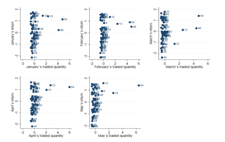
Figure 1
Return versus traded quantity
Source: Developed by the authors.
When focusing on Figure 1, it is clear that two sectors (13 - Various materials and 54 - Gas) had a common characteristic, considering that they maintained returns and traded quantities higher than the average of all the analyzed economic segments. This may mean that they were less impacted by Covid-19 than the others. Also noteworthy is the behavior of sector 12 (Packaging), which in March, after the arrival of the pandemic in Brazil, had a more than proportional drop in its return, remaining below the general average, but maintaining a higher traded quantity than in February. This sector showed a recovery in its returns in the following months.
Finally, it is observed what happened in sector 48 (Pharmaceutical Companies) which, despite maintaining a higher return than the average, suffered a drastic decrease in the traded quantity, mainly in April and May. In the view of Smaniotto and Zani (2020), this downward movement in trading volume was expected in March due to the effects of Covid-19 on the markets.
To carry out a more accurate verification of the economic sectors studied in this work, a cluster analysis of them was developed, in order to identify common characteristics and changes in behavior. Therefore, we sought to determine the appropriate number of clusters using the Calinski-Harabasz pseudo-F. Table 3 presents the results of the Calinski-Harabasz tests for each analyzed month.
| Months | Numbers of Clusters | ||
| 3 | 4 | 5 | |
| January | 87.52 | 9.74 | 85.81 |
| February | 95.66 | 123.33 | 115.86 |
| March | 89.54 | 114.75 | 90.00 |
| April | 72.57 | 81.52 | 66.56 |
| May | 76.58 | 78.50 | 58.83 |
In all performed tests, the Calinski-Harabasz pseudo-F indicated that the ideal number of clusters for the sample presented by this work is four. After dividing the sectors into four groups, it was observed that some remained in the same clusters, regardless of the analyzed moment.
This observation is important, considering the presence of heteroscedasticity in a series of financial returns, where the variance changes over time (Almeida & Ghirardi, 1999).
Tables 4 and 5 show the sectors that remained in the same clusters from January to May 2020.
| Sector Identity | Sector | Standardized Average Return | Standardized Average Traded Quantity | ||||||||
| January | February | March | April | May | January | February | March | April | May | ||
| 2 | Equipment and Services | 0.7271 | 1.0659 | 1.2764 | 1.2679 | 0.8150 | -0.6126 | -0.5163 | -0.5103 | -0.5611 | -0.4777 |
| 5 | Iron and Steel Artifacts | 1.3385 | 1.4796 | 1.1771 | 1.2303 | 0.5177 | -0.3800 | -0.2081 | -0.1222 | -0.0952 | 0.0351 |
| 9 | Various Chemicals | 0.9440 | 0.8311 | 1.0011 | 1.1130 | 1.1499 | 0.1757 | 0.0867 | 0.1101 | 0.4278 | 0.2430 |
| 15 | Heavy Construction | 1.3037 | 1.3229 | 1.3395 | 1.3416 | 1.4492 | -0.4866 | -0.4627 | -0.4738 | -0.5183 | -0.4396 |
| 16 | Consulting Engineering | 1.1982 | 1.2630 | 1.2103 | 1.2038 | 1.3121 | -0.5545 | -0.5110 | -0.4340 | -0.5231 | -0.5088 |
| 21 | Ind. Mach. and Equipment | 1.4145 | 1.3439 | 1.2641 | 1.1907 | 1.4187 | -0.2443 | -0.1277 | -0.1222 | -0.0952 | -0.1381 |
| 22 | Const. and Agric. Mach. and Equipment. | 1.5832 | 1.5027 | 1.7690 | 1.4751 | 1.2604 | 0.0465 | -0.0205 | -0.0226 | 0.1426 | -0.0342 |
| 23 | Weapons and Ammunition | 0.9521 | 1.0869 | 1.1732 | 1.0817 | 0.7276 | -0.6062 | -0.5378 | -0.5269 | -0.5801 | -0.4881 |
| 35 | Yarns and Fabrics | 1.6443 | 1.3650 | 1.2753 | 1.2773 | 1.1234 | -0.2120 | -0.3421 | -0.3245 | -0.3567 | -0.3287 |
| 38 | Hospitality | 1.6176 | 1.5424 | 1.6313 | 1.6341 | 1.5076 | -0.5933 | -0.5244 | -0.5137 | -0.5706 | -0.4846 |
| 45 | Med. and Other Products | 1.4297 | 1.3146 | 1.5362 | 1.5356 | 1.1986 | -0.0828 | -0.0741 | -0.0890 | -0.0001 | -0.0342 |
| 47 | Equipaments | 1.7463 | 1.5992 | 0.8010 | 0.9610 | 1.4463 | -0.2766 | -0.2349 | -0.1553 | -0.1570 | -0.2178 |
As shown in Table 4, cluster 1 is characterized by sectors that maintained above the average returns. However, except for sector 9 (Various Chemicals), the traded quantities were below the average obtained by the others. An interesting characteristic of these sectors is that most of them are linked to the manufacturing industry, except for the hospitality and medicine sectors. The results of the hospitality industry are a surprise, since it maintained an above the average return, even in a moment of extreme crisis, without featuring, according to information from Voglino (2020), among the top twenty assets that had the biggest losses at B3 in 2020.
| Sector Identity | Sector | Standardized Average Return | Standardized Average Traded Quantity | ||||||||
| January | February | March | April | May | January | February | March | April | May | ||
| 13 | Various Materials | 1.3986 | 0.7591 | 0.1240 | 1.3798 | 0.7528 | 2.3404 | 2.3651 | 2.4989 | 2.7671 | 2.6266 |
| 54 | Gás | 1.1347 | 0.8953 | 1.3984 | 1.2228 | 1.3866 | 4.7960 | 4.4826 | 4.7218 | 5.9907 | 6.3752 |
As observed in Table 4, the sectors included in cluster 2 and presented in Table 5 deserve to be highlighted because, in all months, they obtained the highest returns and the largest traded quantities. It is worth noting that sector 9 could not be classified in this cluster, even though it has the same characteristics presented here, because its traded quantities were more than proportionally smaller than those achieved in sectors 13 and 54. The other sectors analyzed did not remain in the same groups to which they belonged in January 2020. It is worth noting that this study raised hypothesis H., that is, Covid-19 did not affect the sectors that makeup B3 in the same way. Therefore, considering the groupings presented in Tables 4 and 5, it could be assumed that they suffered less impact than those that did not fit into the clusters, the latter being possibly more affected by having changed their behavior during the analyzed period in response to the pandemic.
In order to complement the provisions in Tables 4 and 5, Table 6 presents the returns and the average monthly quantities of the sectors that changed clusters during the analyzed period.
| Sector Identity | Sector | Standardized Average Return | Standardized Average Traded Quantity | ||||||||
| January | February | March | April | May | January | February | March | April | May | ||
| 1 | Exploration, Refining, and Distribution | -1.1208 | -1.3294 | -1.4790 | -1.1751 | -0.7028 | -0.3412 | -0.3421 | -0.3743 | -0.3377 | -0.2490 |
| 3 | Metallic Minerals | -0.7544 | -0.7565 | -1.1452 | -1.0250 | -1.2887 | -0.5254 | -0.5003 | -0.4805 | -0.5041 | -0.4361 |
| 4 | Steel | -0.6911 | -0.8488 | -1.0325 | -1.0490 | -0.8675 | -0.5254 | -0.4145 | -0.4307 | -0.4755 | -0.3911 |
| 6 | Copper Artifacts | -1.0475 | -0.9410 | -0.1033 | 0.1462 | -0.1094 | -0.2766 | -0.3153 | -0.2814 | -0.3234 | -0.3287 |
| 7 | Petrochemicals | -0.3707 | -0.5062 | -0.2500 | 0.0531 | 0.1782 | -0.0828 | -0.1277 | -0.0890 | -0.0001 | -0.0342 |
| 8 | Fertilizers and Pesticides | 0.3648 | 1.0232 | 1.0105 | 0.8264 | 0.9148 | -0.3736 | -0.2617 | -0.3677 | 0.2852 | 0.9705 |
| 10 | Wood | 0.6491 | 0.3047 | 1.0741 | 0.4374 | 1.0136 | -0.2120 | -0.3153 | -0.2715 | -0.3329 | -0.2629 |
| 11 | Paper And Cellulose | -0.0151 | -0.1141 | -0.2549 | -0.2483 | 0.2437 | -0.4220 | -0.3689 | -0.3511 | -0.3186 | -0.2074 |
| 12 | Packaging | 1.4439 | 1.3412 | -1.1452 | 0.9805 | 1.5766 | 1.4325 | 1.0785 | 1.3476 | 2.0682 | 1.1784 |
| 14 | Construction Products | -0.0893 | 0.3325 | 0.3237 | 0.1952 | 0.6414 | -0.5965 | -0.5137 | -0.5070 | -0.5801 | -0.4881 |
| 17 | Various Services | -1.3275 | -1.2605 | -0.6936 | -0.6234 | -0.6310 | -0.5674 | -0.5083 | -0.4772 | -0.5421 | -0.4707 |
| 18 | Aeronautical and Defense Material | -0.7924 | -0.7316 | -0.5799 | -1.1438 | -2.0293 | -0.3929 | -0.3582 | -0.3644 | -0.4755 | -0.4881 |
| 19 | Road Material | 0.0651 | 0.1596 | -0.0204 | 0.0485 | 0.0383 | -0.3736 | -0.3421 | -0.4340 | -0.4328 | -0.4326 |
| 20 | Engines, Compressors, and Others | 0.6034 | 0.2134 | 0.5573 | 0.3163 | 0.6762 | -0.4156 | -0.3448 | -0.3279 | -0.3995 | -0.3114 |
| 24 | Air Transport | -1.7549 | -1.5249 | -1.8806 | -1.7508 | -1.5953 | -0.3089 | -0.3153 | -0.4340 | -0.4946 | -0.4465 |
| 25 | Railway Transport | -1.5745 | -1.2472 | -0.8588 | -0.6616 | -0.0611 | -0.4285 | -0.3582 | -0.2847 | 0.1426 | 0.3469 |
| 26 | Waterway Transport | -1.0248 | -1.1886 | -0.6971 | -0.7877 | -0.5889 | -0.3089 | -0.3153 | -0.2549 | -0.2663 | -0.2248 |
| 27 | Road transport | -0.4207 | 0.0397 | -0.3590 | -0.3599 | -0.7967 | -0.0505 | 0.0331 | -0.1222 | -0.1427 | -0.2248 |
| 28 | Highway Exploration | -0.4806 | -0.5501 | -0.1990 | -0.8000 | -0.2110 | -0.3768 | -0.3555 | -0.3279 | -0.3900 | -0.3148 |
| 29 | Agriculture | 0.2900 | 0.2600 | 0.9364 | 0.8047 | 0.7844 | -0.2766 | -0.2617 | -0.2217 | -0.1427 | -0.1381 |
| 30 | Sugar and Alcohol | 0.2900 | 0.4060 | 0.2355 | 0.3971 | -0.2674 | -0.3800 | -0.2617 | -0.3212 | -0.3091 | -0.3148 |
| 31 | Meats and Derivatives | -1.3491 | -1.3646 | -1.4341 | -1.0045 | -1.1463 | -0.3736 | -0.3153 | -0.2880 | -0.1950 | -0.1728 |
| 32 | Beers and Soft Drinks | -1.2128 | -2.1029 | -1.7224 | -1.7160 | -1.4289 | -0.4479 | -0.5083 | -0.4440 | -0.4851 | -0.3980 |
| 33 | Foods | -0.2146 | -0.3882 | -0.0327 | -0.3503 | -0.6383 | 0.4342 | 0.3012 | 0.3423 | 0.5229 | 0.2430 |
| 34 | Incorporations | -0.5151 | -0.3882 | -0.1640 | -0.6791 | -0.6575 | -0.2120 | -0.1277 | -0.2217 | -0.3044 | -0.3183 |
| 36 | Footwear | 0.3213 | 0.4424 | 0.5273 | 0.2387 | 0.1602 | 0.7250 | -0.2349 | -0.2217 | -0.2331 | -0.2490 |
| 37 | Cars and Motorcycles | 0.4692 | -0.0546 | -0.4284 | -0.4753 | 0.2908 | -0.2120 | -0.2617 | -0.3113 | -0.3377 | -0.2455 |
| 39 | Restaurant and Similars | -0.6894 | -0.4337 | -0.0930 | -0.8283 | -0.7449 | -0.4802 | -0.4198 | -0.4208 | -0.5231 | -0.4430 |
| 40 | Educational Services | -0.4883 | -0.4263 | -0.3795 | -0.9523 | -0.8430 | 0.0788 | 0.0867 | 0.0437 | -0.0952 | -0.1035 |
| 41 | Car Rent | -0.1068 | -0.5513 | -1.1811 | -1.5530 | -1.3320 | -0.0828 | -0.1277 | -0.2781 | -0.3567 | -0.3044 |
| 42 | Fabrics, Clothing and Footwear | -0.3059 | -0.1671 | -0.0504 | -0.5367 | -0.7654 | -0.0828 | -0.0741 | -0.0890 | -0.1427 | -0.2074 |
| 43 | Home Appliances | -2.1359 | -2.0745 | -2.3850 | -2.1889 | -2.0397 | -0.4349 | -0.3850 | -0.4042 | -0.3805 | -0.2698 |
| 44 | Various Products | -0.4768 | -0.1874 | -0.0929 | -0.0550 | -0.3635 | -0.2120 | -0.1277 | -0.1553 | 0.0475 | 0.0004 |
| 46 | Medical Services | -0.5509 | -0.2433 | -0.0212 | 0.1122 | -0.1288 | -0.0505 | -0.0473 | 0.0106 | 0.2852 | 0.0697 |
| 48 | Pharmaceutical Companies | 0.2194 | 0.5197 | 0.2738 | 0.3339 | 0.5992 | 4.1498 | 4.7507 | 4.3900 | 0.6180 | 0.4508 |
| 49 | Computers and Equipment | -1.2647 | -1.7224 | -1.5454 | -1.7077 | -1.8966 | -0.5706 | -0.5539 | -0.5336 | -0.6087 | -0.5123 |
| 50 | Programs and Services | -0.9189 | -0.7788 | -0.3076 | 0.2400 | -0.5228 | -0.0182 | -0.0473 | -0.0226 | 0.2852 | -0.1381 |
| 51 | Telecommunications | -0.2372 | -0.1676 | -0.1456 | -0.2633 | -0.3180 | 0.0142 | -0.0473 | 0.0437 | 0.1901 | 0.0697 |
| 52 | Power Generation Companies | -0.2372 | 0.4424 | 0.3870 | 0.3784 | 0.2589 | 0.1757 | 0.0867 | 0.0106 | 0.1426 | 0.0004 |
| 53 | Water and Sanitation Companies | 0.0248 | 0.2756 | -0.4394 | -0.3373 | -0.2250 | 0.4019 | 0.4620 | 0.2096 | -0.0001 | 0.0004 |
| 55 | Banks | -1.0057 | -1.0820 | -1.1811 | -1.1510 | -1.2423 | -0.3089 | -0.3153 | -0.3212 | -0.3282 | -0.3322 |
From Table 6, it is verified that a predominant characteristic of the sectors that changed clusters is that most of them presented, in at least one of the analyzed months, a return below the average. The exceptions to this finding are in sectors 8, 10, 20, 29, 36, and 48. Regarding the average traded quantity, only sectors 12, 33, 48, and 52 showed values above the average in all analyzed periods. Therefore, it can be said that the sectors that have changed clusters, for the most part, were characterized by returns and traded quantities below average.
To check whether H. should be rejected or not, the DID technique was used, having as a milestone the dates of vents involving Covid-19, that is, the first cases and the first deaths that occurred in the United States and Brazil, respectively, as shown in Table 2. It should be noted that the sectors in clusters 1 and 2 were considered as control group; whereas the others (which suffered the most from Covid-19), as treated group.
Table 7 presents the results of the DID's, applying equations (1) and (2), showing the effect of the studied event on the treated group, considering the average returns and the average traded quantities as dependent variables of each analyzed sector, and as the cutoff the dates of the first cases of Covid-19 in the United States and Brazil.
| Dependent | Predictor | Coefficient | Robust Standard Error | T | P>|t| | Confidence Interval |
| Return | DIDUSA | -0.087 | 0.023 | -3.70 | 0.000 | - 0.1323 - 0.0407 |
| Traded Quantity | DIDUSA | -0.052 | 0.025 | -2.07 | 0.038 | - 0.1012 - 0.0028 |
| Return | DIDBrazil | -0.041 | 0.016 | -2.62 | 0.009 | - 0.0713 - 0.0103 |
| Traded Quantity | DIDBrazil | -0.056 | 0.020 | -2.82 | 0.005 | - 0.0948 - 0.0171 |
Before analyzing Table 7, it is worth remembering that Remier and Van Ryzin (2014) teach that the percentages presented in the DID coefficients represent how much the treated group changed concerning the control group, after the occurrence of the analyzed event, in the case of this Covid -19 study. Therefore, it is observed that the first cases that occurred in the United States and Brazil had a more negative impact on the average returns of the treated group than that of the control group. However, the American cases caused a greater reduction, 8.7%, than the Brazilian cases, 4.1%, both being significant at 5% level. About the traded quantity, the negative impact was approximate, being slightly higher in the Brazilian cases, 5.6% compared to the American ones, 5.2%, both with statistical significance of 5% level. These findings confirm what was perceived by Civitarese (2020) when attesting to the negative impact that the confirmation of the first cases had on the returns of B3.
A possible explanation for what is presented in Table 7 is provided by Barbosa, Ribeiro, Consoni, Soares and Frega (2016). The authors state that the economic policy adopted by both the United States and Brazil determines the degree of interdependence between the countries. Also noteworthy are the findings of Chong, Bany-Ariffin, Matemilola and McGowan (2020), when they demonstrate that Brazil is also influenced by the conditions of other markets, such as the Chinese. It is opportune to highlight the indication by Ramelli and Wagner (2020), according to which changes in asset prices can capture the present expectations and that the effects of Covid-19 were also felt in other countries.
Therefore, by the time Covid-19 arrived in Brazil, the market had already created its expectations more than a month before, when the pandemic hit the United States. Empirical proof of this assertion is the information presented by Bomfim (2020), according to which the Ibovespa was not successful in surpassing one hundred thousand points, on July 9, 2020, due to the increase in the number of cases in the United States, which reported sixty thousand new cases of Covid-19 and the possibilities for new quarantines.
Table 8 presents the results of the DID's for the treated group, considering the dates of the news of the first deaths in the USA and Brazil.
| Dependent | Predictor | Coefficient | Robust Standard Error | T | P>|t| | Confidence Interval |
| Return | DIDUSA | -0.022 | 0.015 | -1.47 | 0.142 | - 0.0525 - 0.0076 |
| Traded Quantity | DIDUSA | -0.052 | 0.019 | -2.65 | 0.008 | - 0.8984 - 0.0135 |
| Return | DIDBrazil | -0.024 | 0.015 | -1.60 | 0.111 | - 0.0543 - 0.0056 |
| Traded Quantity | DIDBrazil | -0.054 | 0.019 | -2.81 | 0.005 | - 0.0924 - 0.0165 |
The first deaths resulting from Covid-19 occurred on 03/03/2020 and 03/18/2020, in the United States and in Brazil, respectively. Using these dates as reference, Table 8 shows that the death announcements had a more negative impact on the treated group, both for the return and for the traded quantity. The returns of the treated group were 2.20% and 2.40% lower than the control group, respectively, but they were not statistically significant, since their p-value were higher than 5% significance level. These results seem to contradict the findings of Heyden and Heyden (2020), in stating that the announcements of the first deaths had a greater impact on the stock returns than the report of the first contamination cases, and support the results found by Okorie and Lin (2020 ), when they found that the effect of the virus on returns lasted for a short time, as there was a decrease in the negative impact when comparing the percentages of losses in the first cases with those after the first deaths. On the other hand, there was a decrease in the traded quantities by 5.20% and 5.40%, respectively, both being statistically significant at 5% level.
It is worth mentioning that on the day that the first Covid-19-related death occurred in Brazil, B3 triggered the circuit breaker for the sixth time due to the panic caused by the disease in the market, which reduced the traded quantities. In March alone, this operational procedure was triggered five more times, motivated by factors other than the pandemic, such as the fall in oil prices, capital flight due to market uncertainty, US elections, and the prospect of China's growth being below 6% (Smaniotto & Zani, 2020).
It should be noted that there were three stages of Ibovesba devaluation (10%, 15%, and 20%) that obligated B3 to trigger the circuit breaker (B3, 2020c). One aspect that drew the attention of this research was that all of the companies that were classified in the sectors that made up clusters 1 and 2 were out of the Ibovespa index. Therefore, the aforementioned clusters were not responsible for suspending trading on the stock exchange, but some companies that belong to Ibovespa and that formed the sectors which changed their behavior, possibly due to the advent of the pandemic.
Concerning returns, the results found here were different, at least in terms of statistical significance, from those presented by Al-Awadhi, Al-Saifi, Al-Awadhi and Alhamadi (2020) and El-Basuony (2020). In both studies, the authors found out that the returns are negative and significantly related to the increase in the number of deaths.
Given the above, the hypothesis H. raised in this work, that is, Covid-19 did not affect the sectors that makeup B3 in the same way, could not be rejected since the treated group (which changed its behavior during the analyzed period) suffered a more negative impact from the pandemic. The control group (same behavior during the analyzed period) remained above average, being less affected by the virus.
In order to verify if the clusters had characteristics of a capital market with weak efficiency, the average daily returns of each cluster (treated group, which stayed in the same cluster, and control, which changed from one cluster to another) were calculated and the tests of randomness, normality, and serial correlation were applied to them. Table 9 presents the results found.
| Clusters | Randomness Hypothesis | p-value | Normality Hypothesis | p-value | Serial Correlation Hypothesis | p-value |
| Control | Reject | 0.0004 | Reject | 0.0004 | Reject | 0.3000 |
| Treated | Not reject | 0.7500 | Not reject | 0.2053 | Not reject | 0.1946 |
From the data in Table 9, it was possible to verify that the sectors that make up the treated cluster (groups out of cluster 1 and 2) presented a behavior that matches the prerequisites of a market with weak efficiency, considering that their average daily returns were, at the same time, random, normally distributed and with a low serial correlation between two subsequent trading sessions (current and immediately previous). It is worth mentioning that this conclusion ratifies the behavior perceived by the DID technique, that is, the treated cluster was more affected by the effects of Covid-19 on the capital markets, that is, they responded more quickly to the information that investors had at the time, which made their returns lower than the average for all analyzed companies.
It is worth mentioning the teaching of Rabelo and Ikeda (2004), according to which the positive values of the serial correlations indicate the maintenance of the trends of the average daily returns of the sectors, that is, the control group would be more likely to keep the returns above the average and the treated group, below.
Therefore, the hypothesis H., that was raised in this study, that is, during the analyzed period, there was no verification of weak form of market efficiency in the economic sectors studied, was rejected.
5 CONCLUSIONS
In global terms, the advent of Covid-19 has been the biggest health event in decades. With the resulting crisis affecting people across the globe, it also influences the future of the productive circuit and, as it could not fail to be, the behavior of stock markets on an international scale.
This is a complex phenomenon, multifaceted and full of nuances, however, this does not prevent fractions of this mosaic from being analyzed separately so that specific aspects of this trajectory are properly grasped.
The present article had as a guiding question: “what was the behavior of the sectors that make up B3 concerning Covid-19, about the return and the number of shares traded?”. It was noticed here that, confirming the results of Goodell and Huynh (2020), the sectors behaved differently: those that remained in the same clusters suffered less impact, and the others were subject to greater decreases in their returns and traded quantities. However, the present research observed that the deepening of the disease had no greater impact on the returns of companies' shares, contrary to what was perceived by Rameli and Wagner (2020). Therefore, there was an adjustment of the market as of April 2020. It was also noticed that the number of deaths did not have a statistically significant impact, contrary to what was pointed out by El-Basuony (2020) and Al-Awadhi et al. (2020).
Thus, the hypothesis (H.) that Covid-19 did not affect the sectors that make up B3, in the same way, could not be rejected.
The change in clusters presented by the sectors seems to have been a response to the information that investors had at the time. Thus, the treated group, even though it was more negatively affected by the effects of the pandemic, showed characteristics of a market with weak efficiency. Thus, the hypothesis (H.), according to which there was no verification of an efficient market in the economic studied sectors, during the analyzed period, was rejected.
It should be noted that this study presents as a limitation the fact of promoting a sectorial approach, to the detriment of a focus located on companies. Therefore, it should be considered as an initial step in a research route that must be continuously expanded and refined. Likewise, this gap leaves room for new studies to cover these absences.
Anyway, the study contributed as an empirical evidence that the sectors that makeup B3 showed different behaviors in the face of the new coronavirus pandemic. Most of them felt a hard impact of the disease, which reflected on changes in their average of returns and traded quantities. It was also observed that the companies that formed the sectors that remained in the same clusters also do not participate in the formation of the Ibovespa portfolio, that is, they did not motivate the circuit breakers that occurred in March 2020.
We suggest here that future studies deepen the understanding of the crisis that occurred in March 2020, which triggered the six circuit breakers, and that verify which companies were the most affected, and how Ibovespa behaved concerning the other international indices.
REFERENCES
Al-Awadhi, A. M., Al-Saifi, K., Al-Awadhi, A., & Alhamadi, S. (2020). Death and contagious infectious diseases: Impact of the COVID-19 virus on stock market returns. Journal of behavioral and experimental finance, 27, 100326. https://doi.org/10.1016/j.jbef.2020.100326
Alfaro, L., Chari, A., Greenland, A. N., & Schott, P. K. (2020). (NBER). Aggregate and firm-level stock returns during pandemics in real time. NBER Working Paper, 26950. https://doi.org/10.3386/w26950
Almeida, A., & Ghirardi, A (1999). Estudo comparativo de modelos de gerenciamento de risco de mercado com uma carteira composta por ativos típicos de um fundo de ações. Anais do ENANPAD, Foz do Iguaçu, Brasil, 23.
Assaf, A., Neto. (2003). Mercado Financeiro (3 ed.). São Paulo: Atlas.
B3. (2020a). Setor de atuação. http://www.b3.com.br/pt_br/produtos-e-servicos/negociacao/renda-variavel/empresas-listadas.htm
B3. (2020b). Séries históricas. http://www.b3.com.br/pt_br/market-data-e-indices/servicos-de-dados/market-data/historico/mercado-a-vista/series-historicas/
B3. (2020c). B3 aciona o circuit breaker. http://www.b3.com.br/pt_br/noticias/circuit-breaker.htm
Bao, L., Li, T., Xia, X., Zhu, K., Li, H., & Yang, X. (2020). How does working from home affect developer productivity? - A case study of Baidu during Covid-19 pandemic. Empirical Software Engineering, preprint. https://arxiv.org/pdf/2005.13167.pdf
Baker, S. R., Bloom, N., Davis, S. J., Kost, K. J., Sammon, M. C., & Viratyosin, T. (2020). The unprecedented stock market impact of COVID-19. NBER Working Paper, 26945. https://doi.org/10.3386/w26945
Barbosa, J. D. S., Ribeiro, F., Consoni, S., Soares, R. O., & Frega, J. R. (2016). Impacto do fechamento da bolsa de valores de Nova York (NYSE) sobre o risco de mercado das empresas negociadas na BMFBovespa: um estudo sobre a ótica da interdependência entre mercados. Revista Ambiente Contábil, 8(1), 17-33. https://periodicos.ufrn.br/ambiente/article/view/6567/5987
Blundell, R., & Dias, M. C. (2009). Alternative approaches to evaluation in empirical microeconomics. Journal of Human Resources, 44(3), 565-640. https://muse.jhu.edu/article/466706/pdf
Bomfim, R. (2020). Mercado adia o sonho de retomar patamar do início de março. https://www.infomoney.com.br/mercados/ibovespa-frustra-apos-bater-100-mil-pontos-e-fecha-em-queda-com-temores-de-nova-quarentena-nos-eua/#:~:text=Fechamento-,Ibovespa%20frustra%20ap%C3%B3s%20bater%20100%20mil%20pontos%20e%20fecha%20em,de%20nova%20quarentena%20nos%20EUA&text=S%C3%83O%20PAULO%20%E2%80%93%20O%20Ibovespa%20fechou,acima%20dos%20100%20mil%20pontos
Cardona-Arenas, C. D., & Serna-Gómez, H. M. (2020). COVID-19 and oil prices: Effects on the Colombian peso exchange rate. SSRN Electronic Journal. https://doi.org/10.2139/ssrn.3567942
Cartlidge, J. (2016). Towards adaptive ex ante circuit breakers in financial markets using human-algorithmic market studies. Proc 18th Int. Conf. Artif. Intell. (ICAI), Las Vegas, USA, 18.
Chong, O., Bany-Ariffin, A. N., Matemilola, B. T., & McGowan, C. B., Jr. (2020). Can China’s cross-sectional dispersion of stock returns influence the herding behaviour of traders in other local markets and China’s trading partners? Journal of International Financial Markets, Institutions and Money, 65, 101168. https://doi.org/10.1016/j.intfin.2019.101168
Civitarese, J. (2020). Social distancing under epistemic distress. SSRN Electronic Journal. https://doi.org/10.2139/ssrn.3570298
Culyer, A. J., Newhouse, J. P., Pauly, M. V., McGuire, T. G., & Barros, P. P. (Eds.). (2000). Handbook of Health in Economics. Elsevier.
Dimri, V. (2020). A study on the weak form efficiency of chemicals sector in BSE. International Research Journal of Management Sociology & Humanity, 11(1), 64-73.
Ding, D., Guan, C., Chan, C.M.L., & Liu, W. (2020). Building stock market resilience through digital transformation: using Google trends to analyze the impact of COVID-19 pandemic. Frontier of Business Researc in China, 14, 21. https://doi.org/10.1186/s11782-020-00089-z
El-Basuony, H. (2020). Effect of COVID-19 on the Arab financial markets evidence from Egypt and KSA. IOSR Journal of Business and Management, 22(6), 14-21. https://doi.org/10.9790/487X-2206051421
Evans, M. J., & Rosenthal, J. S. (2004). Probability and statistics: The science of uncertainty. Macmillan.
Fama, E. F. (1970). Efficient capital markets: A review of theory and empirical work. The Journal of Finance, 25(2), 383-417. https://doi.org/10.2307/2325486
Fama, E. F. (1991). Efficient capital markets: II. The Journal of Finance, 46(5), 1575-1617. https://doi.org/10.2307/2328565
Fórum Econômico Mundial. (2020). The Global Risks Reports 2020. Geneva. http://www3.weforum.org/docs/WEF_Global_Risk_Report_2020.pdf
Funakoshi, M., & Hartman, T. (2020). Mad March: How the stock market is being hit by COVID-19. World Economic Forum. Agenda. https://www.weforum.org/agenda/2020/03/stock-market-volatility-coronavirus/
Fundação Getúlio Vargas. (2020). Covid-19 e mercado financeiro. https://fgvprojetos.fgv.br/sites/fgvprojetos.fgv.br/files/mercadofinanceiro_v07.pdf
Goodell, J. W., & Huynh, T. L. D. (2020). Did Congress trade ahead? Considering the reaction of US industries to COVID-19. Finance Research Letters. https://doi.org/10.1016/j.frl.2020.101578
Gormsen, N. J., & Koijen, R. S. J. (2020). Coronavirus: Impact on stock prices and growth expectations. SSRN Electronic Journal. https://doi.org/10.2139/ssrn.3555917
Halpin, B. (2016). Cluster analysis stopping rules in Stata. https://ulir.ul.ie/bitstream/handle/10344/5492/Halpin_2016_cluster.pdf?sequence=2
Hamilton, L. C. (2012). Statistics with Stata: version 12. Cengage Learning.
Haroon, O., & Rizvi, S. A. R. (2020). Flatten the curve and stock market liquidity–an inquiry into emerging economies. Emerging Markets Finance and Trade, 56(10), 2151-2161. https://doi.org/10.1080/1540496X.2020.1785424
Heyden, K., & Heyden, T. (2020). Market reactions to the arrival and containment of COVID-19: An event study. Finance Research Letters, forthcoming. https://doi.org/10.2139/ssrn.3587497
Huo, X. & Qiu, Z. (2020). How does China’s Stock Market React to the Announcement of the COVID-19 Pandemic Lockdown? SSRN Electronic Journal.https://doi.org/10.2139/ssrn.3594062
Jolliffe, I. T., & Cadima, J. (2016). Principal component analysis: a review and recent developments. Philosophical Transactions of the Royal Society A, 374(2065), 20150202. https://doi.org/10.1098/rsta.2015.0202
Kannan, S. P. A. S., Ali, P. S. S., Sheeza, A., & Hemalatha, K. (2020). COVID-19 (Novel Coronavirus 2019) – recent trends. Eur. Rev. Med. Pharmacol. Sci, 24(4), 2006-2011. https://www.europeanreview.org/wp/wp-content/uploads/2006-2011.pdf
Kartal, M. T., Depren, Ö., & Depren, S. K. (2020). The determinants of main stock exchange index changes in emerging countries: evidence from Turkey in COVID-19 pandemic age. SSRN Electronic Journal.https://doi.org/10.2139/ssrn.3659154
Linden, A. (2013). Svysampsi: Stata module for estimating sample size for surveys with a dichotomous outcome variable. http://www.lindenconsulting.org
Liu, H., Manzoor, A., Wang, C., Zhang, L., & Manzoor, Z. (2020). The COVID-19 outbreak and affected countries stock markets response. International Journal of Environmental Research and Public Health, 17(8), 2800. https://doi.org/10.3390/ijerph17082800
Lloyd, C., Prezioso, G., Emigholtz, C., Wintering, J., & Lightbourne, J. (2020). COVID-19: a brief guide to circuit breakers and powers close the market. Alert Memorandum. Clearry Gottlieb Dteen & Hamilton LLP. https://www.clearygottlieb.com/-/media/files/alert-memos-2020/2020_03_20-covid19--a-brief-guide-to-circuit-breakers-and-powers-to-close-the-market-pdf.pdf
Loureiro, C. M. C., Serra, J. P. C., Loureiro, B. M. C., de Souza, T. D. M., Góes, T. M., Neto, J. D. S. A., ... & Marinho, J. M. (2020). Alterações pulmonares na COVID-19. Revista Científica Hospital Santa Izabel, 4(2), 89-99. https://doi.org/10.35753/rchsi.v4i2.175
Ma, C., Rogers, J. H., & Zhou, S. (2020). Global economic and financial effects of 21st Century pandemics and epidemics. SSRN Electronic Journal. https://doi.org/10.2139/ssrn.3565646
Martin, I. W. R., & Wagner, C. (2019). What is the expected return on a stock. The Journal of Finance, (74)4, 1887-1929. https://doi.org/10.1111/jofi.12778
Mehmetoglu, M., & Jakobsen, T. G. (2016). Applied statistics using Stata: a guide for the social sciences. Sage.
Moffatt, P. G. (2015). Experimetrics: Econometrics for experimental economics. Macmillan International Higher Education.
Okorie, D. I., & Lin, B. (2020). Stock markets and the COVID-19 fractal contagion effects. Finance Research Letters, 101640. https://doi.org/10.1016/j.frl.2020.101640
Organização Mundial da Saúde. (2020a). Dados atualizados sobre a Covid-19. https://www.who.int/emergencies/diseases/novel-coronavirus-2019/events-as-they-happen.
Organização Mundial da Saúde. (2020b). Declaração da Covid-19 como pandemia. https://www.who.int/news-room/detail/27-04-2020-who-timeline---covid-19
Pagano, M., Wagner, C., & Zechner, J. (2020a). Covid-19, asset prices, and the Great Reallocation. Voxeu/CEPR. https://voxeu.org/article/covid-19-asset-prices-and-great-reallocation.
Pagano, M., Wagner, C., & Zechner, J. (2020b). Disaster resilience and asset prices.SSRN Electronic Journal. https://doi.org/10.2139/ssrn.3603666
Pevalin, D., & Karen, P. D. J. R. (2009). The Stata survival manual. McGraw-Hill Education (UK).
Rabelo, T. S., Jr., & Ikeda, R. H. (2004). Mercados eficientes e arbitragem: um estudo sob o enfoque das finanças comportamentais. Revista Contabilidade & Finanças, 15(34), 97-107. https://doi.org/10.1590/S1519-70772004000100007
Ramelli, S., & Wagner, A. F. (2020). Feverish stock price reactions to COVID-19. Review of Corporate Finance Studies, forthcoming. https://doi.org/10.2139/ssrn.3550274
Remler, D. K., & Van Ryzin, G. G. (2014). Research methods in practice: Strategies for description and causation. Sage Publications.
Ritchie, H., Ortiz-Espina, E., Beltekian, D., Mathieu, E., Hasell, J., Macdonald, B., Giattino, C., & Roser, M. (2020). Global comparison: where are confirmed deaths increasing most rapidly?https://ourworldindata.org/covid-deaths
Ross, S. A., Westerfield, R. W., & Jaffe, J. F. (2012). Corporate finance. McGraw-Hill Higher Education.
Ruan, C., Liu, J., & Liu. G. (2019). Circuit breakers and market quality: evidence from China. International Journal of Social Science and Economic Research, 4(5), 3597-3604. https://ijsser.org/files_2019/ijsser_04__271.pdf
Seven, U., & Yilmaz, F. (2020). World Equity Markets and COVID-19: Immediate Response and Recovery Prospects. https://mpra.ub.uni-muenchen.de/100987/1/MPRA_paper_100987.pdf
Smaniotto, E., & Zani, J. (2020). Circuit Breakers and Volatility: Evidence from High Frequency Data on Brazilian Stock Exchange. https://www.researchgate.net/profile/Emanuelle_Smaniotto2/publication/342014244_Circuit_Breakers_and_Volatility_Evidence_from_High_Frequency_Data_on_Brazilian_Stock_Exchange/links/5ede9d1c92851cf1386becbf/Circuit-Breakers-and-Volatility-Evidence-from-High-Frequency-Data-on-Brazilian-Stock-Exchange.pdf
Villa, J.M. (2016). Diff: Simplifying the estimation of difference-in-differences treatment effects. Stata Journal, 16, 52-71. https://mpra.ub.uni-muenchen.de/43943/1/MPRA_paper_43943.pdf
Voglino, E. (2020). As 20 ações que mais caíram na bolsa com o coronavírus (até agora). https://comoinvestir.thecap.com.br/acoes-que-mais-cairam-coronavirus-marco-2020/
Yang, Y. H., Shao, Y. H., Shao, H. L., & Stanley, H. E. (2019). Revisiting the weak-form efficiency of the EUR/CHF exchange rate market: Evidence from episodes of different Swiss franc regimes. Physica A: Statistical Mechanics and Its Applications, 523, 734-746. https://doi.org/10.1016/j.physa.2019.02.056
Zhang, D., Hu, M., & Ji, Q. (2020). Financial markets under the global pandemic of COVID-19. Finance Research Letters, 36, 101528. https://doi.org/10.1016/j.frl.2020.101528