Estimating IBNR claims reserve using Gaussian Fuzzy Numbers
Estimação da provisão IBNR usando Números Fuzzy Gaussianos
Estimación de la provisión IBNR utilizando Números Fuzzy Gaussianos
 Ismael Sampaio Bastos ismael@dme.ufrj.br
Leonardo Bruno Vana lbvana@id.uff.br
Carolina Cardoso Novo carolinanovo@id.uff.br
Ismael Sampaio Bastos ismael@dme.ufrj.br
Leonardo Bruno Vana lbvana@id.uff.br
Carolina Cardoso Novo carolinanovo@id.uff.br
Estimating IBNR claims reserve using Gaussian Fuzzy Numbers
Contextus – Revista Contemporânea de Economia e Gestão, vol. 21, núm. 1, Esp., e83343, 2023
Universidade Federal do Ceará

Esta obra está bajo una Licencia Creative Commons Atribución-NoComercial 4.0 Internacional.
Recepción: 25 Enero 2023
Aprobación: 11 Abril 2023
Publicación: 17 Octubre 2023
Abstract: The study aims to present a supplementary approach to the IBNR estimation within the Gaussian Fuzzy Numbers (GFN) framework in alignment with the chain-ladder method. Accordingly, the paper not only introduces concepts and establishes additional perspectives that allow the utilization of this type of fuzzy number in the claim estimation context but also in distinct areas of knowledge. This proposal corroborates the expansion of the fuzzy logic operation in a general sense. The results indicate that the application of the present method offers extensive benefits when compared to the traditional approach and to different types of fuzzy numbers discussed in previous works.
Keywords: claims reserve, fuzzy logic, fuzzy numbers, IBNR, estimating.
Resumo: O estudo teve como objetivo apresentar uma nova abordagem para a estimação da provisão IBNR, usando, para isso, o conceito de Números Fuzzy Gaussianos em consonância com o método chain-ladder. Para tanto, o texto introduz conceitos e estabelece novas perspectivas que possibilitam não apenas a utilização desse tipo de número fuzzy no contexto de provisões técnicas, como também em outras áreas do conhecimento, corroborando assim para a ampliação da adoção da lógica fuzzy de forma geral. Os resultados indicam que a adoção do método proposto oferece grandes benefícios quando comparado à abordagem tradicional e a trabalhos anteriores que exploraram outros tipos de números fuzzy.
Palavras-chave: provisões técnicas, lógica fuzzy, números fuzzy, IBNR, estimação.
Resumen: El estudio tuvo como objetivo proponer un nuevo enfoque para la estimación de IBNR mediante el uso de números Fuzzy Gaussianos en consonancia con el método chain-ladder. Por lo tanto, el texto introduce conceptos y establece nuevas perspectivas que permiten no solo el uso de este tipo de números fuzzy en el contexto de las provisiones técnicas, sino también en otras áreas del conocimiento, contribuyendo así a la expansión de la adopción de la lógica fuzzy en general. Los resultados indican que la adopción del método propuesto ofrece grandes beneficios en comparación con el enfoque tradicional y trabajos previos que exploran otros tipos de números fuzzy.
Palabras clave: provisiones técnicas, lógica fuzzy, números fuzzy, IBNR, estimación.
1 INTRODUCTION
The insurance policy is a contract involving two parts; the policyholder who guarantees the payment of a monetary value referred to as premium, and the insurance company, which ensures a value that will be paid to the policyholder in case of a claim. In order to manage these future payments, a fraction of the premium is required to be directed to compose the claims reserve. According to Mano and Ferreira (2009), claims reserve are values established by companies that assume risk as a product.
It is important to notice that by determining a date t, the claims reserve can be separated into two main parts, Incurred But Not Reported (IBNR) and Reported But Not Settled (RBNS) as presented in Figure 1. The key difference is the fact that IBNR is related to the claims which have not been reported to the insurance company yet, whereas the RBNS refers to the claims previously informed, however, unsettled.

Figure 1.
Claims reserve timeline.
Source: Developed by the authors.
Figure 1 demonstrates that in IBNR, the time interval between the occurrence and the registry of the claim is exclusively considered. Therefore, it is not possible to directly access or determine the values of the reserve without the necessity to establish methods for the estimation.
Furthermore, it is important to observe the application of the word 'registry' instead of 'communication' in the occurrence of the claim in Figure 1. This application was intentional, considering the date the claim is registered on the insurance company system. A discussion regarding this issue can be found in Mano and Ferreira (2009).
Straub and Grubbs (1998) illustrated the idea of IBNR in a case involving a damaged ship in the harbor stating that the damage only became evident when the ship was dry-docked afterwards. In this case, it is possible to notice that a delay may occasionally transpire during the report of the accident and its communication to the insurer. Wüthrich and Merz (2008) cited that when bodily injury and liability occur, it is noticeably common to have an extended length of time before the totality of the circumstances of the claim are clarified and understood.
Carvalho B. and Carvalho J. (2019) highlighted the fact that the constitution of the claim reserves is a major component in the liabilities of a company which assumes operations related to risk. Thus, its correct estimation is a major goal and, in this regard, Mano and Ferreira (2009) emphasized the estimation process relevance of technical provisions. On the one hand, an underestimation could lead the company to civil insolvency, but on the other hand, an overestimation could be problematic to the company due to the fact that the allocation of financial resources in distinct assets instead of technical provisions ought to be avoided. Furthermore, according to the Statistical System of the Superintendence of Private Insurance (SUSEP), at the end of 2022, the IBNR constituted approximately 23% of the total technical provision established in all regional reinsurance companies which highlights the importance of a correct IBNR estimation.
Chukhrova and Johannssen (2017) stated that it is not possible to observe the present value of the accumulated claims on account of the probability that the claims were not correctly reported. Some examples are the cases in which the claim was not partially reported or belated. In this scenario, it is evident the impossibility to determine a real punctual value for the accumulated payments without causing information loss.
Since Fuzzy Numbers are mathematical tools introduced in the context of fuzzy logic to codify vague data as defined in Maturo and Fortuna (2016), the Fuzzy Set Theory utilization allows the actuary not to merely use a single real number but a Fuzzy Number instead, inserting vagueness into the observed value. In accordance with de Andrés-Sánchez (2016), the Fuzzy Set Theory application has the following advantages:
· The estimates are not random variables, consequently, resulting in a difficulty to manipulate arithmetical operations. Contrarily, Fuzzy Numbers are effortless.
· The observations are a consequence of the interaction between the beliefs of the economic agent and the expectations which are exceptionally subjective and vague whether the investigated phenomena is economic or social. The Fuzzy Set Theory is a positive method of managing this information.
· Observations are often not well-defined quantities or confidence intervals which are difficult to handle using non-fuzzy models culminating in information loss.
In the context of Fuzzy Numbers application in the Actuarial Science field, de Andrés-Sánchez and Terceño Gómez (2003), Heberle and Thomas (2014), de Andrés-Sánchez (2016) and, Heberle and Thomas (2016) employed the Triangular Fuzzy Numbers (TFNs) supporting the preference based on the fact that it is simple to work with this type of Fuzzy Number. In contrast, the present work uses the Gaussian Fuzzy Numbers (GFNs) in order to demonstrate that it is not more complicated than the TFNs.
Diversely, the current study demonstrates that the use of GFNs does not infer great difficulty in dealing with this type of FN, in addition, provides tools to work not only in the specific context of claims reserving estimation but also in different areas where data presents vagueness.
This article aims to introduce a new approach to the IBNR estimation applying the Gaussian Fuzzy Numbers (GFNs) concept in consonance with the Chain-Ladder Method (CLM).
2 THEORETICAL FRAMEWORK
As it can be observed in Wüthrich and Merz (2008) research, the CLM was used as a purely computational method for an extended period of time. The work of Mack (1993) established a stochastic foundation in a distribution-free model that serves as basis for the method.
Regarding the fuzzy logic field, it is notable the increase of papers related to insurance since the proposition of the Fuzzy Sets in 1965 by Lofti A. Zadeh. The first publication approaching the use of fuzzy concepts in insurance was performed by de Wit (1982) who developed a study about the employment of Fuzzy Set Theory in underwriting. Subsequently, a number of other insurance themes were studied under the fuzzy logic perspective, namely: insurance pricing, asset allocation funds, and claims reserving estimation. A complete research on the applications of fuzzy logic in the insurance framework can be observed in Derrig and Ostaszewski (1999) and Shapiro (2004).
It is possible to cite as a groundbreaking work, specifically in the claims reserve field, the proposal established by de Andrés-Sánchez and Terceño Gómez (2003) which focused on the application of the fuzzy regression method applying the Triangular Fuzzy Numbers (TFN) to solve actuarial problems including claims reserving estimation. In a similar fashion, de Andrés-Sánchez (2006) and de Andrés-Sánchez (2012) approached the use of fuzzy regression in the estimation.
Apart from the scope of fuzzy regression, it is notable the work developed by Heberle and Thomas (2014) proposing a new method to estimate claims reserve combining CLM with TFN. The paper described the complete methodology and its underlying concepts of the arithmetic operation between triangular fuzzy numbers and the application in the claims reserving estimation process. The main innovation brought by this article is the proposal of a new method that relies on a truly diffused and vastly used method aiming to present a procedure to transfer from the real numbers field to the triangular fuzzy numbers and vice versa.
More recently and similarly, Heberle and Thomas (2016) proposed a new approach to the TFN application by Bornhuetter–Ferguson, however, differently from their previous paper, this one aims to present a procedure to use exogenous information still relying on the Bornhuetter-Fergusson method proposed in their work in 1972.
Since the publication of Antonio and Plat (2013), it is possible to notice a rise in methods to estimate the claims reserve based on individual instead of aggregated data. The main difference is the fact that in individual data every claim is individually considered, nevertheless, the methods that use aggregated data connect individual data at a specific level.
The prime reason for the interest in the utilization of individual data is explained in England and Verrall (2002) which according to the authors, the techniques employing aggregated data were developed before the emergence of desktop computers when these methods were evaluated with pen and paper. However, they raised the question concerning the relation between the constant increase of the computational power and the process of examining the individual instead of aggregated data.
More recently, Delong et al. (2021) examined the use of neural network applied to individual claim data, compared the results with the ones obtained using the chain-ladder method achieving almost equal resulting reserves in both approaches. This information leads to the fact that aggregated models do not imply in the necessity to be simply abandoned and forgotten. As stated by Wüthrich (2018), the CLM is probably the most popular method used as reference for the estimation of the claims reserve due to its simplicity and capacity to generate precise results.
In contrast, machine learning models tend to be more complex and more difficult to implement in practice. In alignment with the model, Carvalho B. and Carvalho J. (2019) highlighted a research carried out in 2016 by the International Actuarial Association (IAA). The study included the participation of 535 members from 42 countries who were inquired in respect of the main methodologies applied for claims reserving estimation. According to the research, the CLM had a widespread performance among the deterministic methods being adopted by 95% of the participants. Specifically in Brazil, the research demonstrated that 97% of the 34 Brazilian insurance companies adopt the CLM as the main or alternative method.
In this article, the proposed method is an extension of the CLM specifically working with GFNs instead of real numbers. This fact will not exceedingly increase the complexity of the method, however, simply changes the procedure that the actuary has to deal with each part of the CLM considering the fuzzy values.
2.1 Chain-ladder method
This section aims to present the CLM with the addition of the concepts presented in Mack (1993). It is important to notice that this article does not make a distinction between the classical chain-ladder method and the chain-ladder model applying CLM in both approaches. The main goal is to resume the data in a structure named run-off triangle where the triangle can be seen as a matrix with each element referring to the number of transpired claims, the total amount of paid claims, or variations in the acquired claims which occurred in the moment and consequently registered with delay following the structure presented in Figure 2.
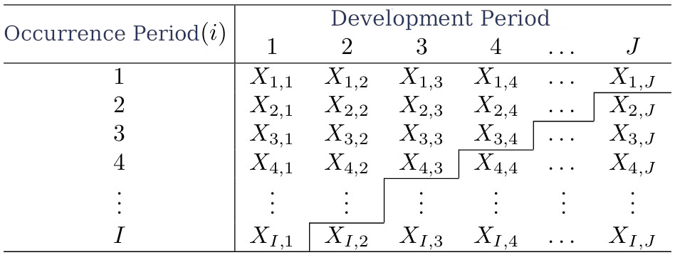
Figure 2.
Development triangle.
Source: Developed by the authors.
In Figure 2, considering the main objective of the claims reserving estimation to determine these values, it is relevant to distinguish the elements which are known in one side and the elements which are not previously recognized on the other. Another important issue to notice is the fact that it can assume different periods of time.
For example, the measurements could last for months and weeks. Similarly, but not mandatory, this article, in order to simplify, only considers the case where the CLM relies in the cumulative triangle sharing the same structure as it can be observed in Figure 3 rather than relying on the incremental triangle; the only difference is that each element is obtained by:
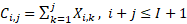 (1)
(1)
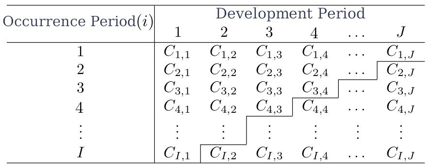
Figure 3
Cumulative development triangle.
Source: Developed by the authors.
According to Wüthrich and Merz (2008), the CLM assumes that the cumulative claims of different occurrence periods are independent and also assumes that exist development factors such as  such as for all
  and all
  we have:
 (2)
(2)The main idea of the chain-ladder method is to infer  using
using  , and using the idea that the claims evolve along the development period according to a factor
  called development factor, being defined as follows:
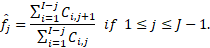 (3)
(3)As it can be observed, Equation 3 presents an estimator proposed in Mack (1993). It is important to mention that, according to Kubrusly et al. (2008), there is a possibility to use other estimators such as the sample mean, the greater factor, the lower factor, the median, or any other statistics. However, this study used the definition proposed in Mack (1993) to simplify the comprehension.
Thus, the values  can be estimated in the following manner:
 (4)
(4)As stated in Mack (1993), the two objectives of chain-ladder method are to estimate:
· The ultimate claim amount
· The outstanding claim reserve 
Where  is defined by the following equation:
 (5)
(5)The chain-ladder method considers that  is not known, for
  . For this reason, it is necessary to estimate
  :
:
 (6)
(6)Where  can be simply estimated by applying Equation 4 with
  .
.
2.2 Fuzzy sets
A fuzzy set  is a collection of pairs
  , where
  is an element of the universe of discourse (
 ) and
) and  denotes the membership grade of
  to
to  , i.e.:
 (7)
(7)where  is called the membership function.
As explained by Zadeh (1965), the concept of the membership function is the point that separates classical from fuzzy logic. Whereas in classical logic if there is a set  and an element
  , only two options stand,
  or
or  ; in fuzzy logic, from a given set
  and element
  , it is possible to say that
  belongs to
  with membership grade
  , where
  can be any value on the interval [0,1].
An example described in de Wit (1982) which occurred in the life insurance field concerning people who drink "a lot" or "a little" alcohol a day. The notion of drinking "a lot" is vague and probably distinct when asking a physician of a life insurance company and a pub owner. In this case, if the set drinking "a lot" was a fuzzy set with a well-defined membership function, this dubiousness would not occur.
According to Bojadziev G. and Bojadziev M. (1995), a fuzzy set is completely defined by its membership function. This definition is moderately useful with great impact considering that if it is given, it is not necessary to describe the whole elements. In this sense, this paper exclusively used the membership function to represent a fuzzy set.
2.3 Fuzzy numbers
As stated in Lee (2004), a fuzzy set is a fuzzy number if it meets the requirements of the following properties:
1. It is defined on  ;
;
2. It is a normalized set;
3. It is a convex set;
4. There is continuous membership function;
5. There is compact support.
As reported by Maturo and Fortuna (2016), it is necessary to add a new property to the list specially dealing with a bell-shaped fuzzy number such as the GFN.
The first property just states that  . Related to property 2, a fuzzy set is called normalized if, and only if exists an element in this set with a membership grade equal to 1, i.e.:
 (8)
(8)In reference to property 3, a fuzzy set is convex if:
 (9)
(9)Considering property 5, a support of a fuzzy set is represented by the following notation:
 (10)
(10)In this sense, when the fuzzy set is referred as containing a compact support, it implies that  is bounded.
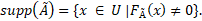
Lee (2004) exposes different types of fuzzy numbers each one with unique characteristics. Figure 4 shows the main fuzzy numbers found in literature where (a) represents a Gaussian Fuzzy Number, (b) represents a Triangular Fuzzy Number and (c) a Trapezoidal Fuzzy Number.
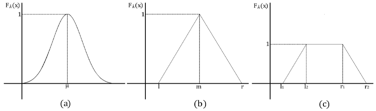
Figure 4.
Examples of Fuzzy Numbers
Source: Developed by the authors.
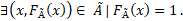
2.4 α-cut sets
An α-cut of a fuzzy set  is composed of the elements that belong to
  that
that  , i.e.:
 (11)
(11)The idea is to merely select a group of elements containing a membership grade greater than or equal to the selected α.
The graphical representation of an α-cut is illustrated in Figure 5. Notably, an α-cut is just a cut held in the fuzzy set, where just elements with membership grade greater or equal to α are extracted.
Figure 5
α-cut set for different type of fuzzy numbers.
Source: Developed by the authors.
2.5 Arithmetic operations between fuzzy numbers
It is possible to notice a number of approaches in arithmetic operations between fuzzy numbers. The present work applied the definition formulated in Hanss (2005). The reason for this approach presents benefits when dealing with symmetric fuzzy numbers, in addition, it simplifies the operations.
Let  and
and  be two symmetric GFNs, the arithmetic operations between them can be defined as follows:
2.5.1 Addition
 (12)
(12)2.5.2 Multiplication
 (13)
(13)It is important to mention that Equation 13 uses the tangent approximation as defined in Hanss (2005). Bearing this in mind, when this type of operation is performed, the symbol = is used instead of  .
.
2.6 Gaussian Fuzzy Numbers
The membership function of a GFN arises from the definition of the Gaussian distribution. According to Heberle and Thomas (2014), from a statistical point of view in this case, the membership function performs a similar role as the probability density function of a random variable.
The probability density function of a Gaussian distribution is defined as follows:
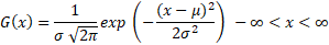 (14)
(14)In that way, Dutta and Limboo (2017) define the membership function of a GFN as:
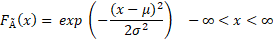 (15)
(15)When following Equation 15 it is possible to admit that a GFN is completely defined by the parameters  and
and  , using for this the notation
  , where
  represents the central value, in other words, the value that has membership degree equals to 1, and
  represents the dispersion of the values concerning
  .
.
The membership function presented in Equation 15 meet the requirements of the first four properties defined at the start of this section, nevertheless, it fails in the last one. It occurs because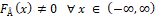 . For this reason, is it not correct to affirm that the GFN presented in fuzzy number. In order to solve this question, it is necessary to adopt the concept of
  -cut, as defined in Maturo and Fortuna (2016).
An  -cut set of a GFN can be described as:
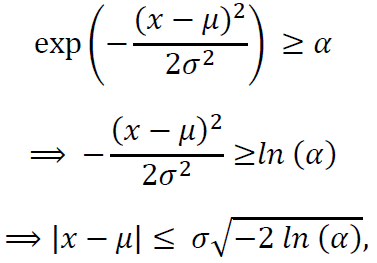 (16)
(16)Thus:
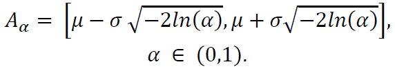 (17)
(17)2.6.1 The uncertainty of a GFN
As illustrated in Gonzalez et al. (1999), the imprecision of a fuzzy number matches with the area below the curve of its membership function. In this respect, it is important to mention the approach performed in Heberle and Thomas (2014) with TFNs where the area of the triangle multiplied by a constant was performed as an uncertainty measure. However, a problem emerges with this definition. The upper limit for the value is boundless culminating in exceptionally great levels of interpretative conditions for the uncertainty. To overcome this scenario, Maturo and Fortuna (2016) proposed, as measurement of the uncertainty, the ratio between the area under the curve of the membership function and its range which culminates in a value contained in [0,1] Indicating the area under the membership function curve as  , the area under the curve of a GFN can be defined as:
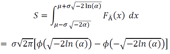 (18)
(18)Representing  , the difference between the upper and lower limit of the interval defined in Equation 17 and
  the uncertainty related to the fuzzy set
  is possible to demonstrate that:
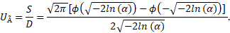 (19)
(19)Alternatively:
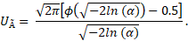 (20)
(20)2.6.2 The expected value of a GFN
While Mano and Ferreira (2009) mentioned the possibility to estimate claims reserve using numeric intervals, de Andrés-Sánchez (2006) states that it is common in practice circumstances the quantification of this interval as a real number. In this sense, it is possible to employ a process named defuzzification. This procedure is frequently adopted to transform a fuzzy number into a real number. As observed in Chakraverty et al (2019), it is possible to note distinct approaches to defuzzification. For example, the Max-Membership Method in which the value with maximum membership grade is exclusively considered. Generally, as stated by the authors, there is a number of defuzzification methods differing by the selected function to translate fuzzy set into a real number. This paper adopts the process defined by de Andrés-Sánchez (2006) and Heberle and Thomas (2014) applying the notion of the expected value of a fuzzy number. Both studies mentioned a previous main focus on TFN and the use of the risk aversion parameter.
In that sense, 𝛽 = 1 means that the decision maker is uncommonly conservative, consequently, indicating the preference to require strong confidence in respect of the estimate being sufficient to ensure future payments even if the company may eventually overestimate it. In counterpart, 𝛽 = 0 indicates that the individual is less cautious, assuming that the lowerst possible value is sufficient to guarantee the solvency of the company. it is worth noting that 𝛽 = 0.5 leads to a neutral position about the risk.
From this perspective, this work aimed to extend to the GFNs the definition elaborated in de Andrés-Sánchez (2006) and in Heberle and Thomas (2014). The definition of the GFN Expected Value is stated as:
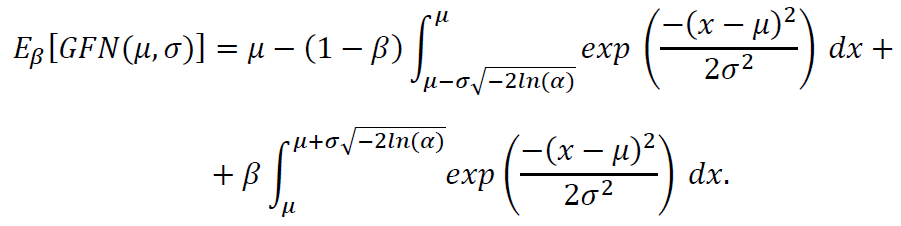 (21)
(21)Alternatively, when applying the cumulative distribution of the standard normal distribution, is possible to rewrite Equation 21 in the following manner:
 (22)
(22)3 METHODOLOGY
In reference to the use of fuzzy numbers in claims reserving estimation, it is possible to highlight the research performed by Heberle and Thomas (2014) applying TFNs to determine the development factors in the chain-ladder method. For that matter, it is worth to point out that despite the widespread utilization of TFNs, a number of disadvantages are presented. According to Maturo and Fortuna (2016), an approach that resorts to TFNs can occasionally reveal an enforced approximation of the real phenomena. Furthermore, it rapidly converges to low values of the membership degree due to their smoothness. As specified in Lee (2004), this characteristic can be observed as a consequence of a TFN membership function being modeled by lines.
Given the above explanation, the utilization of GFNs provides a desirable alternative to model a number of real world circumstances. Thus, it presents smooth variations of the membership values owing to the fact that it is modeled as a bell-shaped curve.
As stated at the beginning of this paper, this study aims to create a fuzzy model to claims reserving estimation using the chain-ladder method as a base. In order to accomplish this goal, it is necessary to adapt the chain-ladder method equations to deal with fuzzy numbers operations.
Considering and assuming that 𝐶̃𝑖𝑗 = 𝐺𝐹𝑁(𝜇𝐶̃𝑖𝑗;𝜎𝐶̃𝑖𝑗), where 𝐶̃𝑖𝑗 is GFN equivalent of 𝐶𝑖𝑗 but in the context of fuzzy numbers, the definition made in Equation 1 is replaced by:
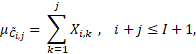 (23)
(23)In addition,
 (24)
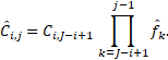
(24)In order to estimate the claims reserve, the Equation 4 is modified as follows:
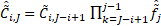 (25)
(25)where 𝑓̃̂𝑗 = 𝐺𝐹𝑁 (𝜇̂𝑓̃̂𝑗; 𝜎̂𝑓̃̂𝑗) and:
 (26)
(26)
 (27)
(27)Due to the fact that Equation 27 is undefined for 𝐼-1, the definition made in Mack (1993) is used in this specific case as stated below:
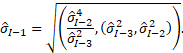 (28)
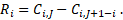
(28)The estimator 𝑅̂𝑗 defined on section 2.1 is therefore represented as a GFN 𝑅̃̂𝑖 = 𝐺𝐹𝑁 (𝜇̂𝑅̃̂𝑖; 𝜎̂𝑅̃̂𝑖) where:
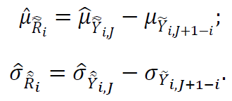 (29)
(29)4 ANALYSIS AND DISCUSSION OF RESULTS
In this section, the results obtained through the application of the methodology defined in the above section were demonstrated. For this purpose, it was used the data from a U.K. Motor Non-Comprehensive account published by Christofides (1997) referring to the total claim amount of paid claims as presented in Table 1.
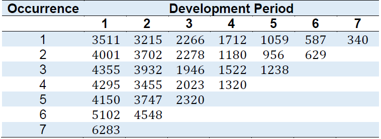
Source: Christofides (1997, D5.17).
Thereby, in order to assemble the chain-ladder method is necessary to work with the cumulative triangle as presented in Table 2.
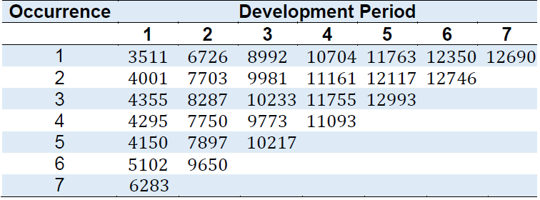
Source: Christofides (1997, D5.16).
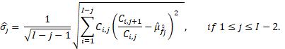
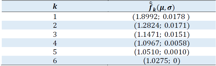
The values presented in Table 2 are utilized for the estimation of 𝑓𝑗 as it can be seen in Table 3. For simplification, the notation (𝜇𝑌̃𝑖𝑗; 𝜎𝑌̃𝑖𝑗) is utilized instead of 𝐺𝐹𝑁(𝜇𝑌̃𝑖𝑗; 𝜎𝑌̃𝑖𝑗).
According to Equation 25, using the table 3 terms, it is possible to determine the unrecognized values of Table 2. In this respect, Table 4 presents the cumulative development triangle.
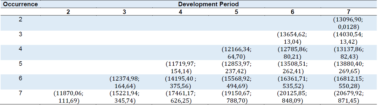
Source: Developed by the authors.
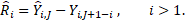
Observing 𝑌̂𝑖,𝑗𝛼 the 𝛼-cut of each set presented in Table 4 is possible to build the 𝛼-cut of estimated fuzzy numbers 𝐶̃̂𝑖𝐽, 𝑖 + 𝑗 > 𝐼 + 1 as presented in Figure 6.
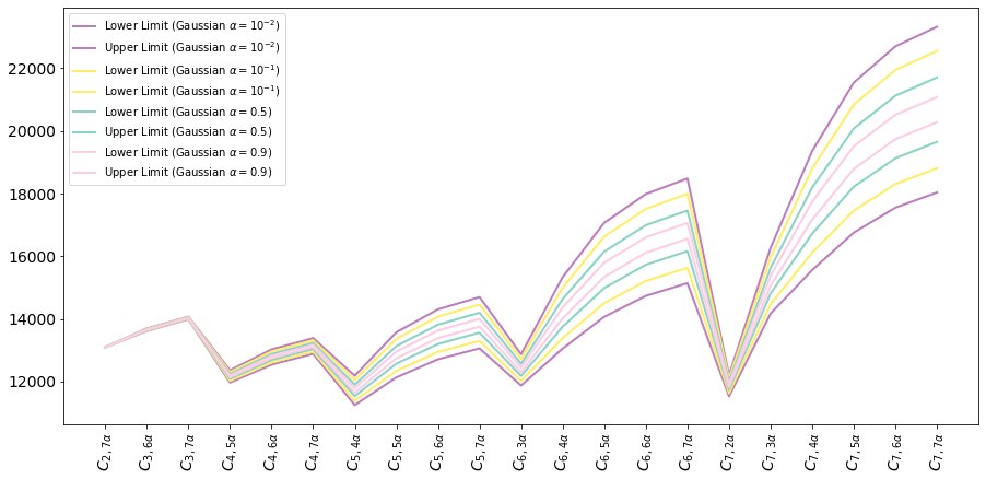
Figure 6
Comparison between 𝛼-cuts for the estimated claims reserve
Source: Developed by the authors.
As observed in Figure 6, the more 𝛼 increases, the lower the range of variation is produced. However, according to Table 5, it is possible to note an increase in uncertainty related to each 𝛼-cut, evidencing the trade-off between precision and uncertainty. This situation occurs due to the fact that when 𝛼 increases, the elementswhich present membership grade lower than 𝛼 are eliminated from the set. Consequently, the lower and upper limits will decrease.
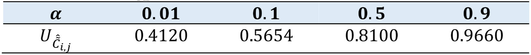
Table 5
Uncertainty of 𝐶̂𝑖,𝑗𝛼 with different 𝛼
Source: Developed by the authors.
The values of Table 5 were obtained through the application of Equation 20. It is important to realize that uncertainty exclusively depends on 𝛼. It is worth mentioning that the intervals presented in Figure 6 are absolutely useful to comprehend the notion of interval where the true value of the claims belong. However, it is occasionally necessary to attribute a real value to the IBNR reserve in practice and not in numeric interval. In this sense, the definition performed in Equation 22 was applied.
Table 6 shows the expected value of 𝑌̃̂𝑖,𝑗 for variations of the parameter 𝛽. The parameter 𝛼 was fixed in 0.01 in order to simplify. It is possible to notice that the greater the risk aversion 𝛽, the greater the expected value. Moreover, when specifically observing the column with 𝛽 = 0.5, it is clear that the result is identical to the one obtained through the classic chain-ladder method which translated into a neutral positioning concerning the risk.
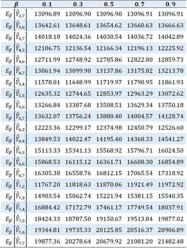
Source: Developed by the authors.
Figure 7 presents the expected value of the claims throughout the years considering β=0.1 and α=0.01.
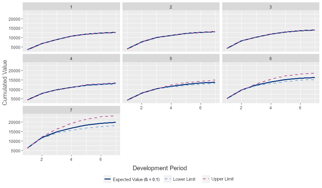
Figure 7
Expected value of paid claims for each occurrence period with β=0.1 and α=0.01
Source: Developed by the authors.
It is evident the approximation of the expected values and the lower limit of the interval displayed in Figure 7, which emphasizes the idea that a lower risk aversion reflects in lower values from the expected value of the estimated claims reserve.
Correspondingly, is it notable the opposite situation considering a risk aversion equal to 0.9 in Figure 8. The expected value is noticeably near the upper limit reinforcing the fact that an acute level of risk aversion leads to an acute estimate of the IBNR.
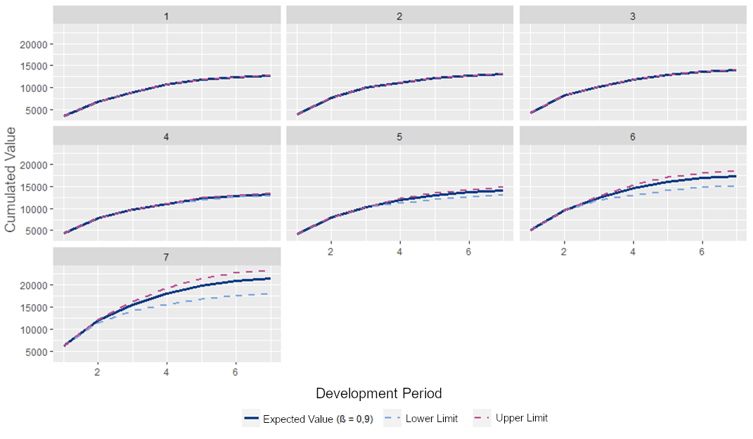
Figure 8
Expected value of paid claims for each occurrence period with β=0.9 and α=0.01
Source: Developed by the authors.
As defined in section 3, it is possible to estimate the outstanding claims reserve. In that sense, the values of 𝑅̃̂𝑖 for each period of occurrence 𝑖 are displayed in Table 7.
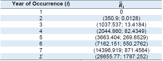
Source: Developed by the authors.
Using the values presented in Table 7 in agreement with Equation 22, it is possible to determine the expected values of the reserves for each year 𝑖 with the correspondent risk aversion parameter 𝛽 as presented on Table 8.
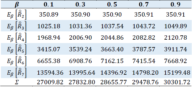
Source: Developed by the authors.
5 EMPIRICAL COMPARISONS WITH SELECTED MODEL
It is clear that the use of the proposed methodology allows the generation of different results depending on the choice of the parameters. Furthermore, it allows to attain the uncertainty related to the obtained interval. However, as described in Heberle and Thomas (2014), the generated uncertainty cannot be misunderstood as stochastic randomness.
Hence, the present section aims to compare the results obtained from the proposed method with the one presented in Heberle and Thomas (2014), where Triangular Fuzzy Numbers were used. There is a necessary remark in relation to the approach made by Heberle and Thomas (2014) about the definition of uncertainty described in the article. That is not a good measure to make comparison because the uncertainty measure proposed by the authors can present values surpassing the magnitude of  . Then, the present paper extents the definition made on Equation 18 to the TFNs instead of using the definition made in Heberle and Thomas (2014).
As a result, the uncertainty of a TFN is constantly equal to 0.5 as demonstrated in Equation 30. Thereby, being 𝐴̃ = TFN (𝑎,𝑙𝑎,𝑟𝑎), its uncertainty 𝑈𝐴̃ is equal to 0.5:
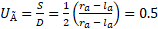 (30)
(30)Following the geometric interpretation, S characterizes the area of the triangle, and D is the length of the base. In this sense, as 𝐴̃ is a fuzzy number, by the property of normality, the height of the triangle is always equal to 1. The reason for the constancy of the uncertainty comes from the fact that a TFN has compact support, which is seen as a disadvantage by Maturo and Fortuna (2016).
From this perspective, the authors cite that if the notion of 𝛼 cut sets is applied to TFNs, the reduction in the uncertainty is proportional to the cut. As a matter of fact, the membership function presents a constant rate of change as it can be observed in Figure 4 (b).
Concisely, the use of Gaussian Fuzzy Numbers allows more freedom as a consequence of the presence of two adjustable factors (𝛼 and 𝛽) while the Triangular Fuzzy Numbers admit only the adjustment of 𝛽. Based on this, Figure 9 presents the results obtained when applying the methodology proposed in Heberle and Thomas (2014) and the results were achieved through the application of the methodology proposed in the present text, both based on the data presented in Christofides (1997).
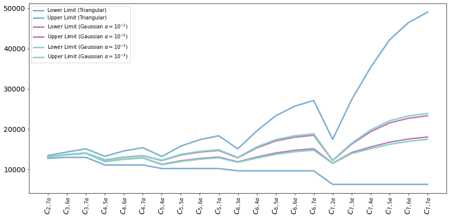
Figure 9.
Comparison between the range of variation for different alpha cuts of GFN and TFN
Source: Developed by the authors.
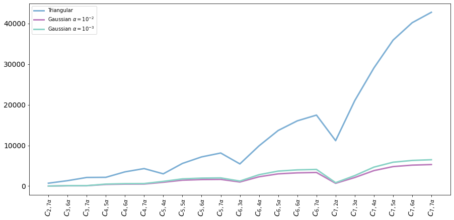
Figure 10.
Comparison between the range of variation for different alpha cuts of GFN and TFN
Source: Developed by the authors.
Observing Figures 9 and 10, is it notable that the result obtained using GFNs presents intervals with lower range of variation and lower uncertainty when compared to the TFNs as observed in Table 9 which reiterates what Maturo and Fortuna (2016) had affirmed. This result evidences the fact that TFNs are occasionally forced approximations of the phenomena as affirmed by the authors.
Table 9 presents the uncertainty for the 𝛼-cuts presented in Figure 7.t is worth mentioning that the uncertainty depends only on 𝛼 so it is not necessary to calculate the uncertainty for every single number. It is clear that the presented 𝛼 -cuts led to lower uncertainty compared to the method using TFNs.
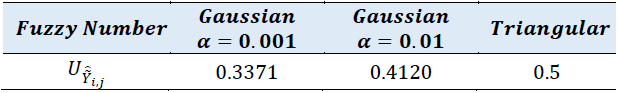
Source: Developed by the authors.
Table 10 displays the overall outstanding claims reserve obtained when applying Equation 29 to the values of Table 4 and to the results using TFNs presented in Heberle and Thomas (2014). It is possible to observe that the use of GFNs generates a lower range of variation as evidenced in Figure 8. However, it is noticeable that TFNs can occasionally assume values that are not consistent in practice, for example 0 and 75474.16.
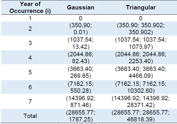
Source: Developed by the authors.
Figure 11 presents the fuzzy numbers of the total outstanding claims reserve using the proposed approach (blue line) and the approach (black line) developed by Heberle and Thomas (2014). The red line represents the 𝛼 chosen, just illustrating the value of 𝛼 is 0.01.
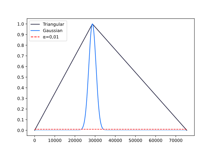
Figure 11
Comparison of the total estimated reserve using GFNs and TFNs.
Source: Developed by the authors.
6 CONCLUSIONS
The present article aimed to present a new approach to the chain-ladder method to estimate the IBNR using Gaussian Fuzzy Number. The results proved that the use of GFNs does not increase the complexity of the model, it simply changes the way that each part is applied.
The results are generated as numeric intervals in which the uncertainty is previously inserted by the definition of the parameter, evidencing an advantage when working with GFNs in comparison with single real numbers. In this context, it is important to evidence that the observed data performed in the empirical tests were not fuzzy, nevertheless, single real numbers instead. This fact demonstrates that the proposed model operates both with real data and fuzzy observations.
A major contribution of the present article is the definition of the expected value allowing the actuary to transit between fuzzy and real numbers. In addition, the definition of uncertainty and the idea of establishing a measure which exclusively outputs values in the specific range is absolutely useful, offering more interpretability of the obtained value.
Another advantage of the approach is the possibility to select the risk aversion level providing flexibility and allowing the adjustment according to the situation and risk aversion of the insurance company in a specific scenario or period.
It is worth mentioning that the results obtained by the proposed approach were consistent presenting identical results compared to the classic chain-ladder method when a neutral aversion to the risk is considered.
When compared to the previous work that made use of TFNs, it is possible to observe that the approach using GFNs presents lower range of variation of the estimated intervals, lower uncertainty and the possibility of the adjustment of the parameter 𝛼, which is a huge advantage, since the uncertainty depends only of 𝛼, while in TFNs this adjustment is not possible.
A gap still maintained is the application of GFNs to other claim-reserving methods such as the Bornhueter-Fergusson which allows questions concerning its advantages and disadvantages when compared to the approach proposed in the current article. Another point that can be explored in a future work is the extension of the presented method to individual claims data.
REFERENCES
Andrés Sánchez, J., & Terceño Gómez, A. (2003). Applications of Fuzzy Regression in Actuarial Analysis. Journal of Risk and Insurance, 70(4), 665-699. https://doi.org/10.1046/j.0022-4367.2003.00070.x
Andrés-Sánchez, J. (2006). Calculating Insurance claim reserves with fuzzy regression. Fuzzy Sets and Systems, 157(23), 3091-3108. https://doi.org/10.1016/j.fss.2006.07.003
Andrés-Sánchez, J. (2012). Claim reserving with fuzzy regression and the two ways of anova. Applied Soft Computing, 12(8), 2435-2441. https://doi.org/10.1016/j.asoc.2012.03.033
Andrés-Sánchez, J. (2016). Fuzzy regression analysis: An actuarial perspective. In C. Kahraman & Ö. Kabak (Eds). Fuzzy Statistical Decision-Making, (pp. 175-201). Springer, Cham. https://doi.org/10.1007/978-3-319-39014-7_11
Antonio, K., & Plat, R. (2013). Micro-level stochastic loss reserving for General Insurance. Scandinavian Actuarial Journal, 2014(7), 649-669. https://doi.org/10.1080/03461238.2012.755938
Bojadziev, G., & Bojadziev, M. (1995). Fuzzy sets, fuzzy logic, applications. World Scientific.
Bornhuetter, R. L., & Ferguson, R. E. (1972, November). The actuary and IBNR. Proceedings of the casualty actuarial Society, 59(112),181-195.
Carvalho, B. D. R. D., & Carvalho, J. V. D. F. (2019) Uma abordagem estocástica para a mensuração da incerteza das provisões técnicas de sinistros. Revista Contabilidade & Finanças, 30(81), 409-424. https://doi.org/10.1590/1808-057x201907860
Chakraverty, S., Sahoo, D. M., & Mahato, N. R. (2019). Defuzzification. Concepts of Soft Computing, 117-127. https://doi.org/10.1007/978-981-13-7430-2_7
Christofides, S. (1997). Regression models based on log-incremental payments. Claims Reserving Manual, Institute of Actuaries Volume 2. D5.16-D5.17.
Chukhrova, N., & Johannssen, A. (2017). State space models and the Kalman-filter in stochastic claims reserving: Forecasting, filtering and smoothing. Risks, 5(2), 30. https://doi.org/10.3390/risks5020030
Delong, Ł., Lindholm, M., & Wüthrich, M. V. (2021). Collective reserving using individual claims data. Scandinavian Actuarial Journal, 2022(1), 1-28. https://doi.org/10.1080/03461238.2021.1921836
Derrig, R. A., & Ostaszewski, K. M. (1999). Fuzzy Sets Methodologies in Actuarial Science. In H. J. Zimmermann (Ed.). Practical Applications of Fuzzy Technologies (pp. 531-553). Springer, Boston, MA. https://doi.org/10.1007/978-1-4615-4601-6_16
Dutta, P., & Limboo, B. (2017). Bell-shaped Fuzzy Soft Sets and Their Application in Medical Diagnosis. Fuzzy Information and Engineering, 9(1), 67-91. https://doi.org/10.1016/j.fiae.2017.03.004
England, P. D., & Verrall, R. J. (2002). Stochastic claims reserving in general insurance. British Actuarial Journal, 8(3), 443-544. http://www.jstor.org/stable/41141552
Gonzalez, A., Pons, O., & Vila, M. (1999). Dealing with uncertainty and imprecision by means of fuzzy numbers. International Journal of Approximate Reasoning, 21(3), 233-256. https://doi.org/10.1016/s0888-613x(99)00024-9
Hanss, M. (2005). Applied Fuzzy Arithmetic: An Introduction with Engineering Applications. Springer.
Heberle, J., & Thomas, A. (2014). Combining chain-ladder claims reserving with fuzzy numbers. Insurance: Mathematics and Economics, 55, 96-104. https://doi.org/10.1016/j.insmatheco.2014.01.002
Heberle, J., & Thomas, A. (2016). The fuzzy Bornhuetter–Ferguson method: an approach with fuzzy numbers. Annals of Actuarial Science, 10(2), 303-321. https://doi.org/10.1017/s1748499516000117
Kubrusly, J., Lopes, H., & Veiga, Á. (2008). Um método probabilístico para cálculo de reservas do tipo IBNR. Revista Brasileira de Risco e Seguro, 4(7), 17-46.
Lee, K. H. (2004). First Course on Fuzzy Theory and Applications (Advances in Intelligent and Soft Computing, 27). (2005th ed.). Springer.
Mack, T. (1993). Distribution-free Calculation of the Standard Error of Chain Ladder Reserve Estimates. ASTIN Bulletin, 23(2), 213-225. https://doi.org/10.2143/ast.23.2.2005092
Mano, C. C. A., & Ferreira, P. P. (2009). Aspectos atuariais e contábeis das provisões técnicas (1st ed.). Escola Nacional de Seguros - Funenseg.
Mano, C. C. A., & Ferreira, P. P. (2018). Aspectos atuariais e contábeis das provisões técnicas (2nd ed.). Escola Nacional de Seguros - Funenseg.
Maturo, F., & Fortuna, F. (2016). Bell-Shaped Fuzzy Numbers Associated with the Normal Curve. In T. Di Battista, E. Moreno & W. Racugno, (Eds.), Topics on Methodological and Applied Statistical Inference (pp. 131-144). Springer, Cham. https://doi.org/10.1007/978-3-319-44093-4_13
Shapiro, A. F. (2004). Fuzzy logic in insurance. Insurance: Mathematics and Economics, 35(2), 399-424. https://doi.org/10.1016/j.insmatheco.2004.07.010
Straub, E., & Grubbs, D. (1998). The Faculty and Institute of Actuaries Claims Reserving Manual. volume 1 and 2. ASTIN Bulletin The Journal of the IAA, 28(2), 287-289. https://doi.org/10.1017/s0515036100012472
Wit, G. (1982). Underwriting and uncertainty. Insurance: Mathematics and Economics, 1(4), 277-285. https://doi.org/10.1016/0167-6687(82)90028-2
Wüthrich, M. V. (2018). Machine learning in individual claims reserving. Scandinavian Actuarial Journal, 2018(6), 465-480. https://doi.org/10.1080/03461238.2018.1428681
Wüthrich, M. V., & Merz, M. (2008). Stochastic Claims Reserving Methods in Insurance. Wiley.
Zadeh, L. (1965). Fuzzy sets. Information and Control, 8(3), 338-353. https://doi.org/10.1016/s0019-9958(65)90241-x