The simplex regression model as a methodology of actuarial analysis
O modelo de regressão simplex como metodologia de análise atuarial
El modelo de regresión simplex como metodología de análisis actuarial
 Jaime Phasquinel Lopes Cavalcante jaime.lopes@ufpe.br
The simplex regression model as a methodology of actuarial analysis
Contextus – Revista Contemporânea de Economia e Gestão, vol. 21, núm. 1, Esp., e83379, 2023
Universidade Federal do Ceará

Esta obra está bajo una Licencia Creative Commons Atribución-NoComercial 4.0 Internacional.
Recepción: 31 Enero 2023
Aprobación: 11 Abril 2023
Publicación: 17 Octubre 2023
Abstract: The risk management business evolves rapidly, so actuaries are faced with the need for new analysis methodologies. However, the use of incorrect methodologies for actuarial modeling can have serious implications for strategic decision making. This study aims to introduce the simplex regression model as a suitable methodology for actuarial modeling of data whose values belong to the unit interval. Using a risk management data set, the linear model with normal distribution and the proposed regression model were compared. The evaluation of the models presented concluded by the quality of the modeling through simplex regression, indicating the quality of this method as a new analysis tool for the actuarial context.
Keywords: regression, simplex, methodology, actuarial, analysis.
Resumo: O mercado de gestão de risco evolui rapidamente, de modo que analistas atuariais são confrontados com a necessidade de novas metodologias de análise. Toda via, a utilização de metodologias incorretas para a modelagem atuarial pode implicar gravemente na tomada de decisões estratégicas. Este estudo busca introduzir o modelo de regressão simplex como uma metodologia adequada para a modelagem atuarial de dados cujos valores pertencem ao intervalo unitário. Fazendo uso de um conjunto de dados sobre gerenciamento de risco, comparou-se o modelo linear com distribuição normal e o modelo de regressão proposto. A avaliação dos modelos apresentados concluiu pela qualidade da modelagem através da regressão simplex, indicando a qualidade deste método como uma nova ferramenta de análise para o contexto atuarial.
Palavras-chave: regressão, simplex, metodologia, atuária, análise.
Resumen: El mercado de la gestión de riesgos evoluciona rápidamente, por lo que los analistas actuariales se enfrentan a la necesidad de nuevas metodologías de análisis. Sin embargo, el uso de metodologías incorrectas para la modelización actuarial puede perjudicar seriamente la toma de decisiones estratégicas. Este estudio pretende introducir el modelo de regresión simplex como metodología adecuada para la modelización actuarial de datos cuyos valores pertenecen al intervalo unitario. Haciendo uso de un conjunto de datos sobre gestión de riesgos, se compararon el modelo lineal con distribución normal y el modelo de regresión propuesto. La evaluación de los modelos presentados concluyó por la calidad de la modelización a través de la regresión simplex, indicando la calidad de este método como una nueva herramienta de análisis para el contexto actuarial.
Palabras clave: regresión, simplex, metodologia, actuarial, análisis.
1 INTRODUCTION
The use of an inappropriate adjustment method in actuarial models can lead to significant losses for companies. This is because actuarial models are used to predict risk and estimate future values such as premiums, reserves, and claims payments. Predictions made by a model that is not properly fitted may be inaccurate, resulting in poor decisions and financial losses (Omari, Nyabura & Mwangi, 2018). For instance, a poorly fitted actuarial model may result in an underestimation of risk, lowering premiums and, consequently, the company's revenue. Similar to underestimating risk, overestimating risk can result in higher premiums, which can drive away customers and cost businesses to rivals. In addition, the lack of a best-fit method can lead to errors in estimating other values, such as loss reserves. If reserves are underestimated, the company may run into financial difficulties in the future because it does not have sufficient funds to pay claims. In order to reduce losses and increase company profits, it is crucial to use a best-fit approach in actuarial models to guarantee that projections and estimates are precise and trustworthy (Erdemir & Karadağ, 2020; Eling & Wirfs, 2019).
Regression analysis is a tool developed in a statistical context and widely used by researchers in various fields of knowledge when the objective is to describe the relationship between a response variable and a set of explanatory variables (Dawes, Green & Sharp, 2018; Sutejo, Pranata & Mahadwartha, 2018; Emirza & Katrinli, 2019; Radaelli & Wagemann, 2019; Arkes, 2020; Nethery et al. 2020). It is observed that the initial proposals of regression models take the form of a linear model whose error term follows a normal distribution with homogeneous variance and the response variable defined as a linear function of independent variables. For example, in the actuarial context, it is possible to use regression to calculate the average amount of the loss sum for different types of insured groups, using group-type indicators as explanatory variables in a regression. Thus, it is possible to use the regression coefficient estimates to determine the relationship between the explanatory variables and the response. Typically, using a regression model requires the inclusion of a hypothesis about the distribution of the response variable. For this reason, loss models and regression are related in the actuarial context (Xie, & Lawniczak, 2018; Lee, Manski, & Maiti, 2020; Rokicki, & Ostaszewski, 2022; Xie, & Luo, 2022).
Even though it is widely used, the classical linear model has limitations in cases where the response variable is non-Gaussian. Other regression models have gradually been developed. In this context, Nelder & Wedderburn (1972) and McCullagh & Nelder (1989) are references for advances in regression models, unifying several model specifications under the flexible class of generalized linear models (GLMs). From this, more appropriate models for various types of responses, such as count, binary and continuous variables, have been developed under the framework of an GLM. Additionally, through this structure, it is possible to model both the mean and dispersion as a function of covariates. The model specification in this class follows generic ways to obtain the likelihood function. This, in turn, allows the estimation of points, intervals, the construction of hypothesis tests, and metrics for model comparison. In other words, using the likelihood function implies obtaining the necessary elements for the practice of statistical modelling.
The incorrect application of the generalized linear model (GLM) in actuarial models might result in inaccuracies in data processing and estimate. GLM is a statistical method for fitting linear regression models to data that do not meet the assumptions of simple linear regression, such as non-normal distributions and non-constant variances. Nevertheless, when attempting to apply GLM to actuarial models, there is a possibility of selecting an incorrect distribution for the data, which might result in erroneous predictions (Hirt & Guevara, 2019). Moreover, using the inappropriate type of link function or explanatory variables might result in models that do not fit the data well, resulting in biased and erroneous estimations. Another typical error is a lack of effective model assessment, such as cross-validation and residual analysis, which can lead to poor model selection and incorrect predictions (Greberg & Rylander, 2022). As a result, it is critical to utilize GLM with caution and to thoroughly examine the model to verify that the predictions are correct and dependable.
Despite their greater flexibility when compared to the classical linear model, generalized linear models have limitations for cases in which the response variable is limited to an interval (a,b), commonly the unit interval (0,1), that is, data that can be expressed as proportions, percentages, rates, or fractions. In this case, extended forms are presented in the literature. Kieschinick & McCullough (2003) point out alternative forms for proposing models with responses belonging to restricted intervals: the classical linear regression model, the Beta and Simplex models and the semiparametric models estimated by quasi-likelihood methods. In this context, Ferrari & Cribari-Neto (2004) provide a more detailed mathematical and computational description of the Beta regression model. Song and Tan (2000) introduced the simplex regression model so that the response variable is assumed to have a simplex distribution. Created by Barndorff-Nielsen and Jørgensen (1991), the simplex distribution was developed from the generalized inverse Gaussian distribution. Some work has been done to model data in the interval (0, 1) using the simplex distribution. Song and Tan (2000) used this distribution to evaluate longitudinal data, assuming that the dispersion parameter is constant, besides presenting relevant properties of this distribution. Song et al. (2004) used this distribution to evaluate longitudinal data under the assumption that the dispersion parameter varies across observations. Venezuela (2007) performed parameter estimation of the simplex model using the generalized estimating equations (GEE) theory.
Miyashiro (2008) studied the simplex regression model with fixed dispersion, presenting model properties and some diagnostic measures. In addition, Santos (2011) developed corrections for the Pearson residual of the simplex model with fixed dispersion and López (2013) used the Bayesian approach for the evaluation of the estimators of the simplex model with variable dispersion. Recently, Oliveira (2015) proposed the nonlinear simplex regression model in addition to presenting some diagnostic measures, and Meireles (2015) proposed two new diagnostic measures constructed from the weighted residuals. Espinheira and Oliveira (2020) presented residuals and influence analyses for the simplex regression model, defining the score vector and the expected and observed information matrices for the model parameters.
In discussing the use of regression models as a tool for actuarial analysis, this research aims to present the simplex regression model as a suitable methodology for actuarial modelling of data whose values belong to the unit interval (0.1). The justification of the theme is based on bibliometric research, which, used the Scopus, Web of Science and CAPES databases. Articles published between the years 2010 and 2022 were considered. The search term "simplex regression model" was combined with the following terms: "actuarial", "actuarial science", "insurance", "risk" in their titles, abstracts or keywords. The search concluded that no articles containing these combinations of search terms were found, thus configuring a window of opportunity for future publications associated with actuarial science. Finally, the rest of this paper is organized as follows. First, drawing on the literature, the main components of the regression model presented are presented. Next, the methodology and the results of the analyses are provided. Finally, the central relationships presented by the method used are discussed.
2 THEORETICAL FRAMEWORK
2.1 The simplex regression model
Similar to the structure and inferential aspects of generalized linear models presented by McCullagh and Nelder (1989), Song and Tan (2000) proposed the class of simplex regression models in which the response variable has a simplex distribution. Defined by Barndorff-Nielsen and Jørgensen (1991), the simplex distribution ( ) is given by
 (1)
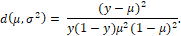
(1)Where 0 < 𝑦 < 1 and 0 < 𝜇 < 1 and 𝜎2 > 0 are the position and dispersion parameters, respectively. In addition, 𝑑 (𝜇,𝜎2) indicates the unit deviation, which is written as
The mean and variance of this distribution are defined respectively by  and
and

where Γ is the gamma function defined as  (Barndorff-Nielsen & Jørgensen; 1991). Once the parameters of this distribution have been set, it is possible to observe that the simplex distribution has a wide range of forms, making it a very flexible distribution for modelling data belonging to the unitary interval (0,1).
The classical simplex regression model assumes that the dispersion parameter is constant over the observations. As in generalized linear models, heteroscedasticity and variable dispersion are distinct from that used in linear models, so variances are not constant since they are defined as a function of the mean. As for linear models, the dispersion parameter is the variance itself. When considering the simplex regression model with variable dispersion, the modelling of the mean and dispersion is performed simultaneously and presented in Espinheira and Oliveira (2020). For this, a regression structure for the dispersion parameter is also presented in addition to the definition of modelling for the mean parameter. The joint estimation of such parameters can be made using the maximum likelihood method.
Assuming  independent random variables, in which each
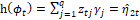
  , has the density shown in (1), then the simplex regression model with varying mean and dispersion satisfies the following functional relations

and
where  and
and  are the vectors of unknown parameters to be estimated,
 and
and  are fixed and known values of the 𝑘 and 𝑞 covariates. Furthermore, the functions g(.) and h(.) are the link functions, which are strictly monotonic and doubly differentiable, such as the logit,
  , probit,
  , with Φ(.) being the cumulative distribution function of the standard normal, log-log,
  , among others. It is important to note that the appropriate choice of link function depends on the type of response variable and the conduct of the study.
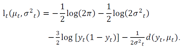
As for the logarithm of the likelihood function, it follows that it is defined as
mong others. It is important to note that the appropriate choice of link function depends on the type of response variable and the conduct of the study.
As for the logarithm of the likelihood function, it follows that it is defined as
The Score vector is obtained by means of the first-order derivatives of the logarithm of the likelihood function. Furthermore, for the composition of the Fisher information matrix for 𝛽 and 𝛾, the second-order derivatives of the logarithm of the likelihood function about the parameters are necessary. These quantities' expressions and matrix forms can be found in Espinheira and Oliveira (2020). In simplex regression models, the maximum likelihood estimators cannot be written in closed form, requiring nonlinear, optimization algorithms. Thus, the initial values used in the iterative scheme must be specified. The reader is advised to read Song and Tan (2000), Espinheira and Oliveira (2020), Espinheira, Silva and Cribari-Neto (2021) and Oliveira, Silva and Espinheira (2022) for more information on the specification of initial values to be used in the iterative scheme.
2.2 Disgnostic and model selection
In order to identify possible disagreements between the assumptions made for the regression model, one of the most relevant steps in modelling is the diagnostic study, commonly performed through the analysis of residuals (Yan, Su & World Scientific, 2009). The effective execution of a model's diagnosis allows the identification of possible extreme values responsible for affecting the result of its adjustment in a disproportionate or inferential way. The definition of residuals for the simplex regression model is performed similarly to the process presented for Generalized Linear Models (GLMs). However, it is verified that the properties of the residuals are not the same, making it essential to define residuals with known properties. Thus, Espinheira and Oliveira (2020) propose and discuss a new residual, weighted residual, in addition to conducting studies of local influence for the diagnostic of simplex regression models.
In the model selection process in simplex regression, one seeks to select regression models with well-explained variance. It is noted that the omission of significant covariates in a regression model commonly results in biases in the estimates of the model coefficients and when a covariate is erroneously entered in the predictors. In this context, it is worth noting the following issues associated with model quality, for example, erroneously modelled dispersion and abandonment of the assumption of non-linearity in the predictors, among others. Finally, a fundamental aspect of regression models is the correct specification of the probability distribution of the response variable, being evaluated using the half-normal probability plot with a simulated envelope presented by Atkinson (1985). A generalization of the criterion 𝑅2 is presented in Nagelkerke (1971), based on using likelihood ratios.
3 METHODOLOGY
Aligned with the objective of this study, an application in which the simplex regression model can be used as an actuarial analysis method will be presented. The actuarial question addressed in this application refers to the cost-benefit ratio of risk management (measured in percentages) about certain asset losses, such as industry size and type. For this purpose, the data used came from the studies by Schmit and Roth (1990). The data comprise a sample size of n=73, which was collected from a questionnaire sent to risk managers of large organizations based in the United States. After controlling for company variables like company size and industry type, the study's goal was to associate cost efficiency to management philosophy in reducing the firm's exposure to various property and casualty losses. The description of the data is as follows:
| Variable | Description |
| FIRMCOST | Response variable (a percentage). Represents the company's risk measure. |
| ASSUME | Retention amount per occurrence as a percentage of total assets. |
| CAP | It indicates whether the insurance company is licensed to provide coverage for itself. |
| SIZELOG | Logarithm of total assets. |
| INDCOST | A measure of the insurance company's segment risk. |
| CENTRAL | A measure for assessing the amount of risk to be retained. |
| SOPH | A measure of the degree of importance in the use of analytical tools. |
To obtain a better understanding of the data, we will first look at the fundamental summary statistics in Table 2. The largest value of the dependent variable FIRMCOST is 0.975, which is more than five standard deviations above the mean.
| Variable | Mean | Median | Standard Deviation | Minimum | Maximum |
| FIRMCOST | 0.110 | 0.061 | 0.162 | 0.002 | 0.975 |
| ASSUME | 2.574 | 0.510 | 8.445 | 0.000 | 61.820 |
| CAP | 0.342 | 0.000 | 0.478 | 0.000 | 1.000 |
| SIZELOG | 8.332 | 8.270 | 0.963 | 5.270 | 10.600 |
| INDCOST | 0.418 | 0.340 | 0.216 | 0.090 | 1.220 |
| CENTRAL | 2.247 | 2.200 | 1.256 | 1.000 | 5.000 |
| SOPH | 21.192 | 23.00 | 5.304 | 5.000 | 31.000 |
Data analysis revealed that this point is observation 15. Moreover, two further observations of the variable FIRMCOST had unusually large values, observations 16 and 72, resulting in a right-skewed distribution. Table 3 displays the correlations between the independent variables and the dependent variable FIRMCOST. Only the variables SIZELOG and INDCOST showed a considerable degree of linear correlation with the variable under consideration (FIRMCOST).
| FIRMCOST | ASSUME | CAP | SIZELOG | INDCOST | CENTRAL | SOPH | |
| FIRMCOST | 1.000 | 0.039 | 0.088 | -0.366 | 0.326 | 0.014 | 0.048 |
| ASSUME | 0.039 | 1.000 | 0.231 | -0.209 | 0.249 | -0.068 | 0.061 |
| CAP | 0.088 | 0.230 | 1.000 | 0.196 | 0.122 | -0.004 | -0.087 |
| SIZELOG | -0.366 | -0.209 | 0.196 | 1.000 | -0.102 | -0.079 | -0.209 |
| INDCOST | 0.326 | 0.249 | 0.122 | -0.102 | 1.000 | -0.084 | 0.093 |
| CENTRAL | 0.014 | -0.068 | -0.004 | -0.080 | -0.085 | 1.000 | 0.283 |
| SOPH | 0.048 | 0.062 | -0.087 | -0.201 | 0.093 | 0.283 | 1.000 |
The modelling of the response variable is considered using the generalized linear model, whose distribution of the response variable has a normal distribution, and the simplex regression model with variable dispersion. After the evaluation of the variables on the model, the potential models for the study were defined as follows
 [Model 01]
 [Model 02]
and

The first model was used to evaluate the fit under the assumption of normality of the data, i.e., the generalized linear model with normal distribution and identity-type link function was adopted. Then, the second model was defined to study the simplex regression model with variable dispersion. The link functions used were: log-log, for the mean submodel and log, for dispersion modelling. Model quality was assessed utilizing residual analysis and selection criteria. Finally, the computational operations and preparation of the graphs presented in this study were performed using the R programming, data analysis and graphics environment in its version 4.0.3, available at http://www.R-project.org .
4 ANALYSIS AND DISCUSSION OF RESULTS
Starting with model 01, we sought to verify the quality of the fit of the data presented to investigate the assumption that the linear model, commonly used in actuarial practices (Frees, 2012), would be suitable for the analysis of the data set presented. Table 4 presents the parameter estimates, standard errors (s.e) and the p-values of Wald's test for the nullity of the coefficients (p-value). The results of the estimates in this modelling allowed us to infer that the intercept (responsible for the slope of the straight line equation) and the covariates used were statistically significant at the nominal 5% level.
Through this, it was possible to verify the relationship between the estimated parameters and the average response, the variable FIRMCOST (a measure of the company's risk). Thus, as the response variable is increased by one unit of percentage, the positive relationship between the variable FIMRCOST and the intercept was observed, as well as between the variable FIMRCOST and INDCOST. Additionally, the comparison between the response variable and the covariate SIZELOG evidenced a negative linear relationship, indicating that the increase in one unit of percent in the response variable implies the reduction of the SIZELOG variable, that is, as the risk increases the logarithm of total assets is reduced.
However, a superficial analysis of the model, i.e., a study based only on the estimated parameters' significance, could indicate that model 01 is adequate for the study and inferences about the analyzed data set could be inappropriately made. Therefore, in contexts where the analysis of the parameter estimates indicates an apparent quality of the data modelling, diagnostic techniques play a crucial role in validating the inferential aspects of the model. In this case, the Figure 1 presents the analysis of the residuals and the simulated envelope of model 01. The graphical analysis pointed to severe problems in this modelling, i.e., through the graphs it was observed the presence of potentially atypical points (Figure 1 (a)), indications of high variability in the data set, indicating that the modelling assuming a heteroscedastic structure would be more appropriate. This fact could be proven through the simulated envelope (Figure 1 (b)), responsible for indicating the inappropriateness of the normal distribution for modelling the data and the need for modelling the dispersion of the data. Another critical aspect to note is the poor quality of modelling data in the unit interval using the normal distribution since data restricted to the unit interval generally exhibit asymmetry and have a specific pattern of heteroscedasticity.
| Description of parameters | beta1 (const.) | beta2 (Sizelog) | beta3 (Indcost) | |
| Full Dataset | Estimate | 0.4881 | -0.0564 | 0.1563 |
| s.e | 0.1563 | 0.0178 | 0.0794 | |
| p-value | 0.0026 | 0.0023 | 0.0076 | |
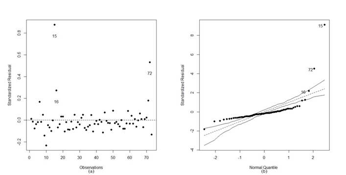
Figure 1
Plots of the residuals and simulated envelope. - Model 01.
Source: Elaborated by the author.
Given the signs of heteroscedasticity and the non-suitability of the normal distribution, we tried to model the data using model 02. Table 5 presents the parameter estimates, standard errors (s.e) and p-values of the Wald test for the nullity of the coefficients (p-value). Unlike model 01, it was found that the values for the intercepts (const.) were not statistically significant at the nominal 5% level. Then, by diagnosing the postulated model (Figure 2(a)), the presence of the points {15.72} was observed as potentially influential. In the second model, the observation {16} could not be highlighted as a possible influential point, indicating an improvement in the modelling.
| Description of parameters | beta1 (const.) | beta2 (Sizelog) | beta3 (Indcost) | gama1 (const.) | gama2 (Sizelog) | gama3 (Indcost) | |||
| Full Dataset | estimate | 0.4788 | -0.2491 | 2.265 | -2.5177 | 0.5528 | 2.6032 | ||
| s.e | 0.2902 | 0.0282 | 0.2315 | 1.5258 | 0.1739 | 0.7748 | |||
| p-value | 0.0989 | 0.000 | 0.000 | 0.0989 | 0.0015 | 0.0008 | |||
| Points {15.72} deletes | estimate | 0.7654 | -0.2622 | 1.1851 | -4.1639 | 0.8026 | -0.0072 | ||
| s.e | 0.2673 | 0.0268 | 0.1837 | 1.6879 | 0.1935 | 0.8681 | |||
| p-value | 0.0042 | 0.000 | 0.000 | 0.0136 | 0.0000 | 0.0000 | |||
Moreover, through the analysis of the simulated envelope (Figure 2(b)), the occurrence of such points, especially observation {15}, negatively impacted the quality of the fit of the distribution of the model's response variable, in this case, the simplex distribution, which even with the presence of atypical observations presents a better fit, in terms of distribution, when compared with the model that assumes the normality of the response variable (model 01).
The model was re-estimated by excluding the points {15.72} to verify the assumption that the inferential impact of the potentially atypical points affects the parameter estimates. Since the percentage changes in the parameter estimates caused by removing the points were low, it was clear that the points were atypical, i.e., outliers. However, the variability exerted by these points on the model structure is reduced, allowing the model to present an excellent fit to the data. This quality can be observed by comparing the graphs of residuals and especially the simulated envelopes, where it is verified that the simplex distribution is suitable for modelling the response variable (Figure 3).
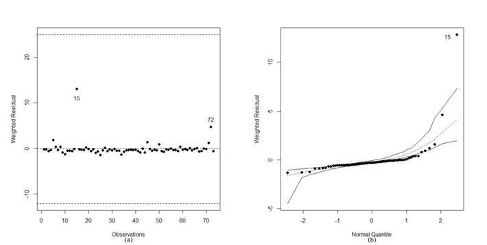
Figure 2
Plots of the residuals and simulated envelope. Model 02 - Full Dataset.
Source: Elaborated by the author.
As for the interpretation of the parameters that make up the submodel of the mean of model 02 with the excluded observations, it should be noted that the interpretation was made on the log-log link function. Thus, the interpretation followed in terms of the increase in risk, i.e., the response variable, the firm's risk, will increase by about 0.769 per unit of the logarithm of total assets (INDCOST) when the other covariates are kept fixed. Additionally, for the covariate INDCOST, it was observed that firm risk would grow by about 3.271 per unit associated with the covariate. Thus, it was observed that the growth of total assets and a higher level of uncertainty associated with the insurance companies segment, covariates LOGSIZE and INDCOST, are significant for the increase of the measure linked to risk management.
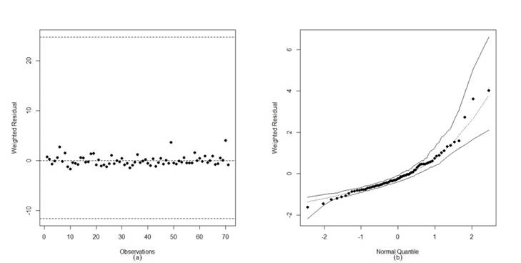
Figure 3.
Plots of the residuals and simulated envelope. Model 02 - Points {15,72} deleted.
Source: Elaborated by the author.
For comparison purposes, the normal and simplex distributions were used to model the data set without considering the effect of covariates. Table 6 shows the value of the likelihood functions of the distributions studied.
| Null model | Model with covariates | |
| Simplex | 73.596 | 112.39 |
| Normal | 29.973 | 38.9611 |
Through the values presented, when using this measure as a comparison criterion, it was possible to corroborate with the other measures presented in the study, i.e., the measures point to the low quality of modelling according to the use of the generalized linear model and emphasizes the quality of the simplex regression model. In addition, another criterion that corroborated with the quality of the simplex regression model was the pseudo-𝑅2 of Nagelkerke, where the variability explained by the simplex regression model with all observations was 0.6545, or 65.45%. Still, considering the removal of atypical observations, an 𝑅2 equal to 67.68% was obtained. For the model considering the regression based on a normal linear model, the criterion presented a value of 23.07%.
5 CONCLUSIONS
When it comes to actuarial models, adopting the wrong adjustment approach might result in huge losses for businesses. This is due to the importance of actuarial models in projecting risk and calculating future values like as premiums, reserves, and claims payments. When a model is not correctly modified, the predictions it produces might be erroneous, resulting in poor judgments and financial losses. Of concern, the adoption of an ineffective technique might result in inaccuracies in the calculation of other critical parameters, such as loss reserves. When reserves are understated, the firm may experience financial problems in the future since it will not have enough cash to satisfy claims. To prevent these problems, it is critical to use actuarial models in a "best-fit" manner, ensuring that forecasts and estimations are accurate and dependable. This method allows the organization to cut losses while increasing earnings.
Actuarial scientists play a critical role in measuring ordinary actuarial occurrences in the context of risk analysis and risk management. Utilizing empirical data to predict and manage risk allows businesses to make educated decisions and prevent financial losses. Actuaries can assess the probability of occurrence of events like as claims, fatalities, sicknesses, and retirements using mathematical and statistical models. Furthermore, the financial and risk management markets are continually changing, posing new problems to actuarial analysts. Many actuarial practitioners are faced with the necessity to create new techniques of analysis as financial risks become more complicated and consumer expectations shift. To assist market needs, actuaries must stay current on trends and advancements in their profession in order to assure the accuracy and efficiency of the actuarial models employed by businesses. Hence, selecting a "best-fit" strategy might be critical to a company's financial performance. Thus, this study aimed to present the simplex regression model as a methodology for actuarial applications.
The implementation of appropriate statistical models is critical to ensuring the precision of estimates and, as a result, risk avoidance. Several frequently used models, however, may be inefficient for modeling data with specific properties, such as heteroscedasticity or response variables contained in a single interval.The application related to risk management, it was possible to verify that the simplex regression model, directed to modelling data in the unit interval, presented a better data fit when compared to the generalized linear model with normal distribution, a widely used methodology, but which presents low efficiency when used in modelling data whose response variable is contained in the interval (0,1) and data with heteroscedasticity presence. As a result, the simplex regression model stands out as a practical way for modeling data in the unit interval.
Another aspect being highlighted is the use of diagnostic techniques since defining the quality of a model based only on the significance levels of the estimated parameters may configure a severe error in inferential terms. Through the diagnostic graphical analysis, it was possible to identify the presence of potentially influential points, observe the behaviour of the randomness of the residuals and the correct specification of the probability distribution of the response variable. Using the selection criterion based on Nagelkerke's pseudo-𝑅2, the modelling using simplex regression with variable dispersion presented a high capacity to explain the variance of the estimated model, standing out concerning the GLM with normal distribuition.
Given the results presented, simplex regression models are suitable for actuarial modelling in cases where the response variable is contained in the unit interval and the presence of heteroscedastic patterns. Thus, this study achieves its general objective by presenting the main aspects of this regression methodology in an actuarial context. As for the limitations of this work, one can cite the use of secondary data and the fact that the application does not present a case associated with the Brazilian risk market. In addition, given the lack of studies with this type of modelling in actuarial sciences, this study lays the foundation for the following future works: application of the simplex model to the evaluation of Brazilian data sets, from the perspective of loss ratio analysis and the study of the nonlinearity assumptions of the parameters estimated by the regression model.
Acknowledgments
The author would like to thank the two anonymous reviewers for their valuable contributions to the improvement of this work and the Coordination for the Improvement of Higher Education Personnel (CAPES Foundation) for the doctoral scholarship.
REFERENCES
Arkes, J. (2020). Teaching Graduate (and Undergraduate) Econometrics: Some Sensible Shifts to Improve Efficiency, Effectiveness, and Usefulness. Econometrics, 8(3), 1-36. http://doi.org/10.2139/ssrn.3427791
Atkinson, A. C. (1981). Two graphical display for outlying and influential observations in regression. Biometrika, 68, 13-20. https://doi.org/10.1093/biomet/68.1.13
Dawes, J., Kennedy, R., Green, K., & Sharp, B. (2018). Forecasting advertising and media effects on sales: Econometrics and alternatives. International Journal of Market Research, 60(6), 611-620. https://doi.org/10.1177/1470785318782871
Eling, M., & Wirfs, J. (2019). What are the actual costs of cyber risk events?. European Journal of Operational Research, 272(3), 1109-1119. https://doi.org/10.1016/j.ejor.2018.07.021
Emirza, S., & Katrinli, A. (2019). The relationship between leader construal level and leader-member exchange relationship: The role of relational demography. Leadership & Organization Development Journal, 40(8), 845-859. https://doi.org/10.1108/LODJ-02-2019-0084
Erdemir, Ö. K., & Karadağ, Ö. (2020). On comparison of models for count data with excessive zeros in non-life insurance. Sigma Journal of Engineering and Natural Sciences, 38(3), 1543-1553.
Espinheira, p. L., & Oliveira, A. (2020). Residual and influence analysis to a general class of simplex regression. TEST, 29, 523–552. https://doi.org/10.1007/s11749-019-00665-3
Espinheira, P. L., Silva, L.C.M., & Cribari-Neto, F. (2021). Bias and variance residuals for machine learning nonlinear simplex regressions. Expert Systems With Applications, 185, 1-13. https://doi.org/10.1016/j.eswa.2021.115656
Ferrarri, S. L. P., & Cribari-Neto, F. (2004). Beta regression for modelling rates and proportions. Journal of Applied Statistics, 31, 799-815. https://doi.org/10.1080/0266476042000214501
Frees, E.W. (2012). Regression Modeling with Actuarial and Financial Applications (1 ed.). Cambridge: Cambridge University Press.
Guillen, M., Bermúdez, L., & Pitarque, A. (2021). Joint generalized quantile and conditional tail expectation regression for insurance risk analysis. Mathematics and Economics, 99, 1-8. https://doi.org/10.1016/j.insmatheco.2021.03.006
Greberg, F., & Rylander, A. (2022). Using Gradient Boosting to Identify Pricing Errors in GLM-Based Tariffs for Non-life Insurance. Stockholm, Sweden.
Hirt, E. R., & Guevara, H. R. (2019). Forecasting and prediction. In Handbook of research methods in consumer psychology, 241-258, Routledge.
Kieschinick, R., & Mccullough, B. D. (2003). Regression analysis of variates observed on (0,1): percentages, proportions and fractions. Statistical Modelling, 3(3), 193-213. https://doi.org/10.1191/1471082X03st053oa
Lee, G., Manski, S., & Maiti, T. (2020). Actuarial applications of word embedding models. ASTIN Bulletin: The Journal of the IAA, 50(1), 1-24. https://doi.org/10.1017/asb.2019.28
Liu P., Yuen K.C., Wu L.C., Tian G.L., & Li T. (2020). Zero-one-inflated simplex regression models for the analysis of continuous proportion data. Statistics and Its Interface. 2020; 13(2), 193-208. https://doi.org/10.4310/SII.2020.v13.n2.a5
López, F. O. (2013). A Bayesian Approach to Parameter Estimation in Simplex Regression Model: A compararison with Beta Regression. Revista Colombiana de Estadística, 36, 1-21. http://www.scielo.org.co/scielo.php?script=sci_arttext&pid=S0120-17512013000100001&lng=en&tlng=en
Mccullagh, P., & Nelder, J. A. (1989). Generalized Linear Models (02 ed.). London: Chapman and Hall.
Meireles, L. C. (2015). Coeficientes de Predição para os Modelos de Regressão Beta e Simplex (Master’s dissetation). Federal University of Pernambuco, Recife, PE, Brazil.
Miyashiro, E. S. (2008). Modelos de regressão beta e simplex para análise de proporções (Doctoral thesis). University of São Paulo, São Paulo, SP, Brazil.
Nagelkerke, N. J. D. (1991). A note on a general definition of the coefficient of determination. Biometrika, 78(3), 691-692. https://doi.org/10.1093/biomet/78.3.691
Nelder, J. A., & Wedderburn, R. W. M. (1972). Generalized linear models. Journal of the Royal Statistical Society, 135, 370-384. https://doi.org/10.2307/2344614
Oliveira, A. (2015). Regressão Simplex Não Linear: Inferência e Diagnóstico (Master’s dissetation). Federal University of Pernambuco, Recife, PE, Brazil.
Oliveira, A., Silva, J., & Espinheira, P. L. (2022). Bootstrap-based inferential improvements to the simplex nonlinear regression model. PLOS ONE, 17, 1-27. https://doi.org/10.1371/journal.pone.0272512
Omari, C. O., Nyambura, S. G., & Mwangi, J. M. W. (2018). Modeling the frequency and severity of auto insurance claims using statistical distributions. Journal of Mathematical Finance, 8, 137-160. https://doi.org/10.4236/jmf.2018.81012
Radaelli, C.M., & Wagemann, C. (2019). What did I leave out? Omitted variables in regression and qualitative comparative analysis. Eur Polit Sci, 18, 275-290. https://doi.org/10.1057/s41304-017-0142-7
Rokicki, B., & Ostaszewski, K. (2022) Actuarial Credibility Approach in Adjusting Initial Cost Estimates of Transport Infrastructure Projects. Sustainability 2022, 14. https://doi.org/10.3390/su142013371
Santos, L. A. (2011). Modelos de Regressão Simplex: Resíduos de Pearson Corrigidos e Aplicações (Doctoral thesis). University of São Paulo, São Paulo, SP, Brazil.
Schmit, J.T., & Roth, K. (1990). Cost effectiveness of risk managements practice. The Journal of Risk and Insurance, 57(3), 455-470. https://doi.org/10.2307/252842
Song, P. X. -K., & Tan, M. (2000). Marginal models for longitudinal continuous proportional data. Biometrics, 56, 496-502. https://doi.org/10.1111/j.0006-341X.2000.00496.x
Song, P. X. -K., Qiu, Z., & Tan, M. (2004). Modelling heterogeneous dispersion in marginal models for longitudinal proportional data. Biometrical Journal, 46, 540-553. https://doi.org/10.1002/bimj.200110052
Sutejo, B.S.,Pranata, Y.K.N., & Mahadwartha, P.A. (2018). Demography factors, financial risk tolerance, and retail investors. Atlantis Press.
Venezuela, M. K. (2007). Equação de estimação generalizada e influência local para modelos de regressão beta com medidas repetidas (Doctoral thesis). University of São Paulo, São Paulo, SP, Brazil.
Wulff, J.N., & Villadsen, A.R. (2020). Keeping it within bounds: Regression analysis of proportions in international business. J Int Bus Stud, 51, 244-262. https://doi.org/10.1057/s41267-019-00278-w
Wu, X., Nethery, R.C., Sabath, M.B., Braun, D., & Dominici, F. (2020). Air pollution and COVID-19 mortality in the United States: Strengths and limitations of an ecological regression analysis. Science Advances, 6(45). https://doi.org/10.1126/sciadv.abd4049
Xie, S., & Lawniczak, A. (2018). Estimating Major Risk Factor Relativities in Rate Filings Using Generalized Linear Models. International Journal of Financial Studies, 6(4), 84. https://doi.org/10.3390/ijfs6040084
Xie, S., & Luo, R. (2022). Measuring Variable Importance in Generalized Linear Models for Modeling Size of Loss Distributions. Mathematics, 10(10), 16-30. https://doi.org/10.3390/math10101630
Yan X., Su X., & World Scientific (Firm). (2009). Linear regression analysis: theory and computing (1 ed.). Singapore: World Scientific Pub.