Low-cost Data Acquisition System for Deformation Determination with Accelerometers
Sistema de adquisición de datos de bajo costo para determinación de deformaciones con acelerómetros
 Daniela Desiderio Maya danieladmaya@outlook.com
 Orlando Susarrey Huerta osusarrey@yahoo.com
Juan Carlos Suárez Calderón jcarlos.suarez@live.com
Iván Rocha-Gómez ivanrocha.go@gmail.com
Orlando Susarrey Huerta osusarrey@yahoo.com
Juan Carlos Suárez Calderón jcarlos.suarez@live.com
Iván Rocha-Gómez ivanrocha.go@gmail.com
Low-cost Data Acquisition System for Deformation Determination with Accelerometers
Científica, vol. 27, núm. 2, pp. 1-16, 2023
Instituto Politécnico Nacional
Recepción: 05/02/2023
Aprobación: 24/05/2023
Abstract: In this article, a proposal for a data acquisition system specifically designed to evaluate fracture failure caused by vibration in an electrical harness bracket in a commercial vehicle is presented. The proposed system is a low-cost open architecture solution that allows comprehensive data collection, visualization, and analysis. The data captured by the accelerometers are sent to the microcontroller for processing and subsequent analysis using MATLAB software. In order to validate the proposed system, tests were performed using five different conditions on the vehicle. The electrical harness bracket was instrumented in the area where the fracture failure occurs to evaluate its performance under different scenarios. In addition, a stress analysis was carried out on the harness material, and the results obtained through the presented data acquisition system were compared, which demonstrated its effectiveness and the obtaining of satisfactory results. This research represents a significant advance in the detection and analysis of vibration failures in electrical harnesses, providing a useful tool for the validation of commercial vehicles.
Keywords: data acquisition system, accelerometers, open architecture, vibrations, vibration analysis.
Resumen:
En este artículo, se presenta una propuesta de sistema de adquisición de datos diseñado específicamente para evaluar la falla por fractura causada por vibración en un bracket de un arnés eléctrico en un vehículo comercial. El sistema propuesto es una solución de arquitectura abierta de bajo costo que permite la recolección, visualización y análisis exhaustivo de los datos. Los datos capturados por los acelerómetros son enviados al microcontrolador para su procesamiento y posterior análisis utilizando el software MATLAB. Con el fin de validar el sistema propuesto, se realizaron pruebas utilizando cinco condiciones distintas en el vehículo. Se instrumentó el bracket del arnés eléctrico en la zona donde se presenta la falla por fractura, para evaluar su desempeño bajo diferentes escenarios. Además, se llevó a cabo un análisis de esfuerzos en el material del arnés, y se compararon los resultados obtenidos mediante el sistema de adquisición de datos presentado, lo cual demostró su eficacia y la obtención de resultados satisfactorios. Esta investigación representa un avance significativo en la detección y análisis de fallas por vibración en arneses eléctricos, proporcionando una herramienta útil para la validación de vehículos comerciales.
Palabras clave: sistema de adquisición de datos, acelerómetros, arquitectura abierta, vibraciones, análisis de vibraciones.
I. Introducción
Data acquisition systems are essential in different industries because it is important to test the components and systems to know if works properly. This tool allows engineers to collect and analyze data from various sensors and sources. In the automotive industry, these systems are utilized to measure parameters such as temperature, pressure, and vibration in critical components of vehicles, including engines, suspensions, and brakes. With the increasing complexity of modern vehicles, data acquisition systems have become more sophisticated, providing more accurate and precise measurements to support engineering and design decisions. The analysis of data acquired from these systems is crucial in ensuring the safety, reliability, and performance of automotive components and systems.
In the last 15 years, data acquisition systems have been developed for applications where real-time monitoring is important, such as research [1] carried out where a monitoring and acquisition system is carried out of data applied to decentralized renewable energy plants with a USB interface. Also, with real-time monitoring, another data acquisition system applied to a production management system was carried out [2], complementing this study with a man-machine interface. On the other hand, the fact that a system consists of an open architecture allows the user to be able to add or replace components that are compatible with the system in order to create a more powerful system. Unlike those offered by corporations that are only compatible with their own equipment of the same brand. By having an open architecture, there is a decrease in system costs. An example is the one created with a [3] Raspberry Pi as a low-cost data acquisition system for human-powered vehicles, where tests on a bike as a test vehicle having performance comparable to higher priced systems.
The applications of data acquisition systems are unlimited, in order to mention one, we have [4] the prevention of failures, the predictive capacity of preventive and predictive maintenance, the improvement of the quality of the machined product, and the reduction of failure times and [5] or the one developed for obtaining.
In the analysis of deformations to find faults in systems from different fields of science, more methods have been investigated to be applied depending on the system and obtain precise results. In 2001 [6], an approximate deformation analysis and a FEM analysis for the incremental bulging of metal sheets using a spherical roll was carried out. This application was used for a machine that performs a wide range of metal forming metal sheets of complex shapes, which exemplifies that the most appropriate method of obtaining deformations is selected according to the application.
Subsequently, [7] in an investigation, more than 100 studies regarding the analysis of discontinuous deformations were reviewed, classifying the studies into 3 groups: (a) validation with respect to analytical solutions, (b) validation with with respect to results of other numerical techniques, and (c) validation with respect to laboratory and field data. This data collection is important to know which methods have been used in the analysis of deformations depending on the application. There are three main techniques for strain validation: qualitative evaluation, which visually examines the runtime behavior of the simulations; semi-quantitative evaluation, which compares the numerical results of the simulations, and quantitative evaluation, where the numerical results of the simulation are evaluated in detail with respect to similar analytical, laboratory or field results. Having a previous simulation generates cost savings to detect possible failures in a system and creates security in the system. For example, one important application in this area was [8] for simulations of earthquake-induced landslides.
In recent years, the study of deformations in structures has been proposed, which has become relevant. For example, [9] the proposed investigation of the monitoring of deformation of architectural structures through three-dimensional laser scanning and the Finite Element Method, creating a model that can be applied in constructions. New methods have been developed for the measurement of deformations [10], such as the one carried out to determine the plastic deformation and the fracture behavior of polypropylene compounds, where he proposes a measurement method of strain defining an intrinsic flow stress equation by varying strain rates in propylene compounds. For the design, the study of the deformations continues over time since it is essential to know the working limits of a component.
II. Methodology
For the design, creation, and validation of the data acquisition system, the methodology shown in Fig. 1 was followed.
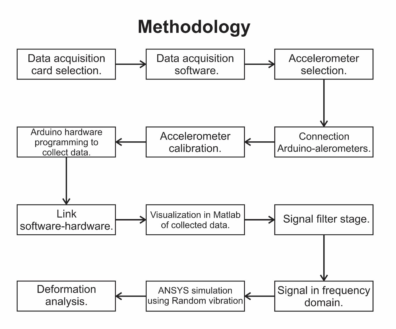
Fig. 1.
Data acquisition system methodology.
For the card selection, we considered the following parameters: Number of analog inputs: Each analog input can read one sensor, so it is important to consider the desired number of sensors when selecting a card.
Interface
Resolution: It is represented by the number of discrete values in which an analog-to-digital converter can translate an analog signal to digital and is measured based on the number of bits that the card has. The number of bits represents the maximum number of discrete values that an analog-to-digital converter can have.
To calculate these discrete values, equation (1) is used:
 (1)
(1)Where:
n: is the number of bits of resolution of the card.
Dv: Discrete values.
For voltage, resolution is described in equation (2):
 (2)
(2)Where:
VR= Voltage Resolution [V].
OR= Operating Range [V].
D. Sampling frequency: The sampling of analog signals has some conditions so that information losses do not occur. The sampling ratio can be defined as equation (3):
 (3)
(3)Where:
t: sampling time [s].
N: number of samples.
Fm: sampling rate [Hz].
According to Nyquist's sampling theorem, "Given a function whose energy is entirely contained in a bandwidth, if it is sampled at a frequency equal to or greater than the original function, it can be fully recovered by means of an ideal low-pass filter."
The minimum sampling frequency required to make a quality digital recording must be equal to twice the maximum frequency of the analog signal to be digitized. As expressed in equation (4):
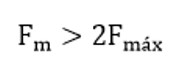 (4)
(4)Where:
Fm= sampling frequency [Hz].
Fmáx = maximum frequency [Hz].
As illustrated in Figure 2, the yellow wave is a frequency that coincides at specific points with the original frequency (in blue) but does not represent the initial wave.
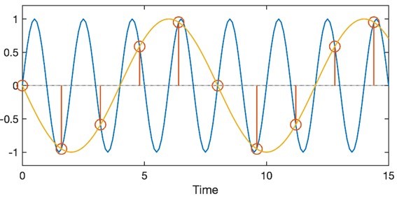
Fig. 2.
Aliasing effect.
Architecture type: the architecture of a card is the relationship that it can have with the different components that make up the system in which it is interacting. This architecture can be open or closed.
An open architecture card allows you to add, modernize, and change its components, even if they are from a different manufacturer. In contrast, a closed architecture card is where the hardware manufacturer chooses the components, and they are typically not upgradable.
In accordance with the criteria for creating a data acquisition system, the parameters shown in Table 1 compare the cards.
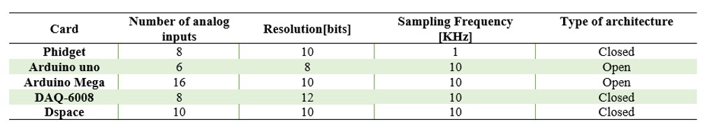
The selection of cards for data acquisition is the Arduino Mega card. The main factor is that it has 16 analog inputs, and in this project, 12 inputs are required because it is necessary to use 4 accelerometers, and each one of these needs 3 pins that are on the "x", "y" and "z" axes. Another important factor is the type of architecture since it is possible to integrate components from other manufacturers.
To calculate the resolution voltage, it is substituted in equation 2, considering that the Arduino Mega card has a 10-bit resolution and an operating range of 3.3 V. Obtaining what is described in the equation (5):
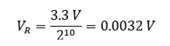 (5)
(5)This resolution is an accurate representation of the signal generated for data acquisition.
The Nyquist sampling theorem must be fulfilled in order not to present the aliasing phenomenon. Therefore, according to the calibration of the commercial vehicle engine, a change is made in the gearbox at a maximum of 3000 rpm. The conversion from rpm to Hertz is shown in equation (6).
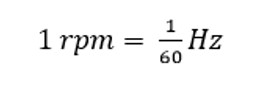 (6)
(6)To carry out the conversion to Hz, it is substituted in equation (6), obtaining what is shown in equation (7):
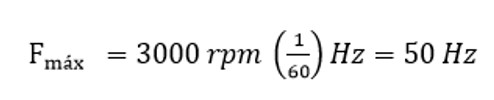 (7)
(7)According to the sampling frequency of the Arduino Mega card, the inequality of the Nyquist theorem equation (4) is satisfied, shown in equation (8):
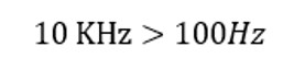 (8)
(8)Fulfilling Nyquist's theorem, the Arduino mega card is the right one for data acquisition.
The accelerometer selected in this system is the ADXL335, as it has a measurement range for vibration frequencies up to 200 Hz. Considering that the range of the maximum sampling frequency is 50 Hz, the sensor can perform the measurement. The specifications of the accelerometer are shown in Table 2.
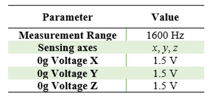
The selected accelerometer, the measurement range complies with the maximum measured frequency (50Hz), in addition to using the 0 value of each axis to determine the range of values in which the measurements will be oscillating.
For data acquisition, it was carried out by means of 2 software: Arduino and Matlab ®. The Arduino software was used to perform the data acquisition and was linked to Matlab® to graph the data obtained, while an Excel file was generated to store such data, as illustrated in Fig. 3.
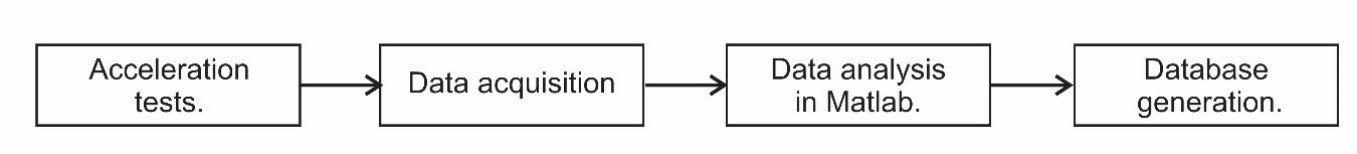
Fig. 3.
Data acquisition flow chart.
III. Tests
For the tests, the battery was instrumented with 4 accelerometers, as shown in Fig. 4, with the objective of knowing the vibrations at each strategic point close to the end where the electrical connector presents the fault.
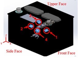
Fig. 4.
Instrumented battery with accelerometers.
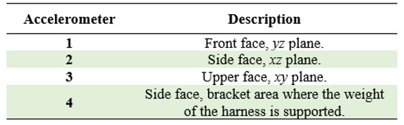
Table 3 describes each position of the accelerometers on the battery and the electric bracket.
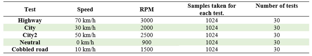
For the test cases, 5 different paths are considered with the speed that would be applied given the operating conditions. A total of 150 tests were performed, which are described in Table 4. Each type of test was replicated under the same conditions 30 times to obtain reliable measurements.
For each type of test, the average measurements were obtained, and a graph was made for each accelerometer. Fig. 5 shows the graphs of the average data of the highway test.
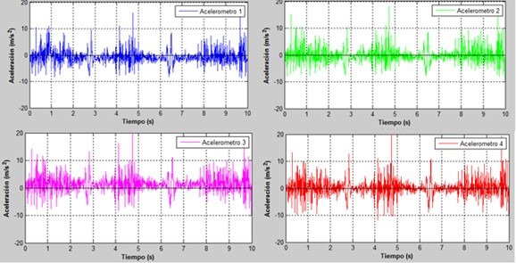
Fig. 5.
Average acceleration data graphs of each accelerometer the Highway test.
For the city test, the average data obtained from the 30 tests carried out was considered and graphed, as shown in Fig. 6.
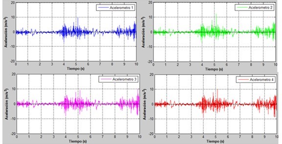
Fig. 6.
Average acceleration data graphs of each accelerometer the City test.
The same procedure was carried out for the data obtained in the east of City2; the average data of the 30 tests carried out were graphed with the results shown in Fig. 7.
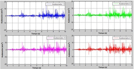
Fig. 7.
Average acceleration data graphs of each accelerometer the City2 test.
The data obtained from the neutral test were averaged over the 30 tests, and the average data shown in Fig. 8 were plotted.
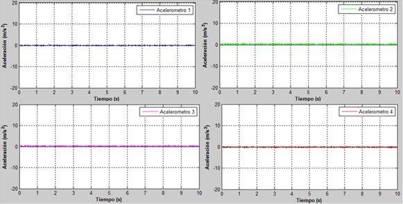
Fig. 8.
Average acceleration data graphs of each accelerometer for the Neutral test.
Finally, the data of the paved road were considered, averaging the 30 tests carried out and graphed as shown in Fig. 9.
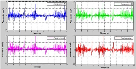
Fig. 9.
Average acceleration data graphs of each accelerometer the Cobbled Road test.
IV. Data processing
For the treatment of the signal, a filter was applied since the generated signals have noise. In order not to lose information in the signal, the filter that was chosen was a digital type of Infinite Impulse Response (IIR). Since it is for a discrete signal and compared to a Finite Impulse Response (FIR) type, the former requires fewer memory locations for its realization. On the other hand, the IIR filter is more efficient in terms of computation time, and the response is of finite duration since if the input remains at zero for some consecutive periods, the output will also be zero.
When analyzing the signals with a filter, it is concluded that there is no loss of information since the eliminated peaks are abnormal values that are not repetitive in all the measurements.
Additionally, the IIR filter can exhibit sharper roll-off characteristics, making it suitable for this application that requires efficient filtering and preservation of signal features. Behind, IIR offers feedback, allowing for the creation of recursive filters that can effectively handle dynamic signals and adapt to changing conditions.
To obtain the graphs in the frequency domain and perform a modal analysis of the frequencies exhibited in the system, the Fourier Transform was applied. By computationally using the Fast Fourier Transform, it decomposes the signals into the frequencies that were present in the measurements, each with its amplitude and phase.
Within the analysis of the frequency spectrum graphs, it is found that the greatest amplitudes of all the frequencies are found in accelerometer 4. This accelerometer is in the bracket area where the weight of the harness is supported. Fig. 10 shows all the frequency domain graphs of the accelerometer 4.
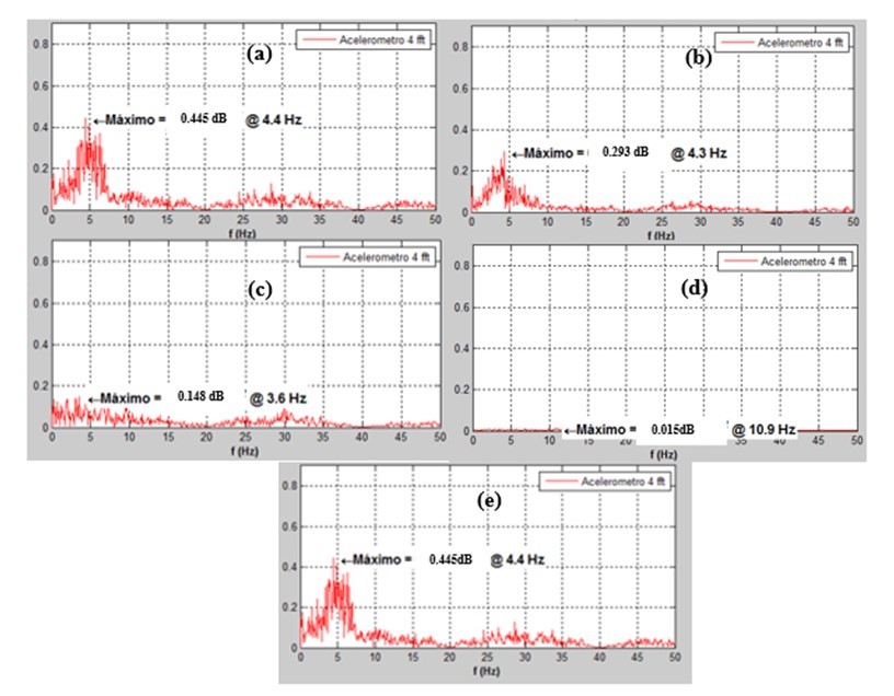
Fig. 10.
Graphs in the frequency domain of the accelerometer 4 of the tests: (a) Highway, (b)City, (c)City2, (d)Neutral, and (e)Cobbled Road.
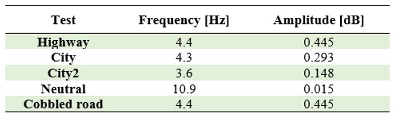
The overall spectral content of the signal has the highest density at distributed frequencies of 1-12 Hz in all tests. Table 5 shows the maximum values obtained in the frequency domain graphs in each test, with the lowest frequencies presenting the maximum values.
V. Data processing
To find out if the part of the electrical support of the battery is failing due to vibrations, the part was subjected to an analysis in ANSYS called Random Vibrations to find out the equivalent stress with the processed data from the frequency domain of the tests: Highway, City, City2, Neutral and Cobbled Road.
Random vibration analysis is used to evaluate stresses and deformations in a system that is subjected to vibrations. This approach [11] is based on the study of random vibrations, that is, at unpredictable frequencies that do not repeat themselves. It is applied in real-world situations where the vibrations do not follow a pattern. Randomness becomes a fundamental characteristic of the excitation or input of this analysis. To carry out this analysis, it is carried out with the mode superposition method.
The mode superposition method is a technique used in structural analysis to determine the dynamic response of a system by combining individual vibration modes. To obtain this, it is broken down into fundamental vibration modes, and the response of each mode is considered separately. When obtaining the response of each mode, they are superimposed to calculate the total response of the system.
For the mathematical modeling of the mode superposition method, the equation of motion is considered and can be expressed as:
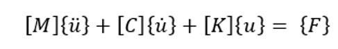 (9)
(9)Where:
[M]= structural mass matrix
[C] = structural dampling matrix
[K] = structural stifness matrix
= nodal acceleration vector
= nodal velocity vector
{u(t)} = nodal displacement vector
{F} = the time-varying load vector
Often, the matrix form is obtained from the discretization of a physical problem using the finite element method. If N denotes the number of degrees of freedom, the matrices have the size NxN.
A prerequisite for a mode superposition is to calculate the eigenfrequencies and the shapes of the corresponding modes. Using the eigenvalue equation, we have:
 (10)
(10)Where:
ω =natural frequency
A small number n of the eigenfrequencies is calculated. The result of this calculation is a set of natural frequencies (ωi) with corresponding (ui) mode shapes, where i ranges from 1 to n. where the eigenmodes are orthogonal with respect to the mass and stiffness matrices. This means that:
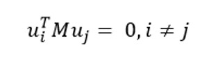 (11)
(11)and
 (12)
(12)The orthogonality relation can be described as:
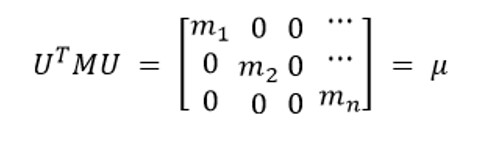 (13)
(13)Where:
mn= eigen modes
The diagonal elements are called modal masses. The values of the modal masses depend on the normalization of the eigenmodes. This normalization is arbitrary since the mode only represents a shape, and the amplitude has no physical meaning. Therefore, mass matrix normalization is performed. Where the eigenmodes are scaled so that each mi= 1, giving:
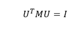 (14)
(14)Where:
I = Identity matrix
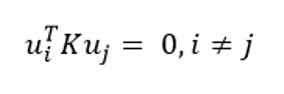
The corresponding orthogonality relation for the stiffness matrix is:
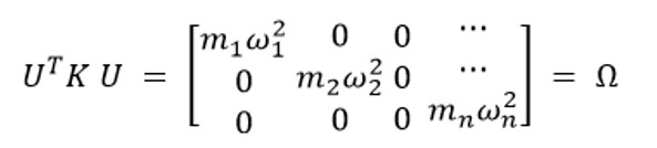 (15)
(15)Using mass matrix normalization, the diagonal matrix consists of the natural angular frequencies squared. The basic approach to mode superposition is that the displacement can be written as a linear combination of the eigenmodes:
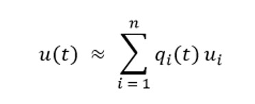 (16)
(16)Where:
qi= modal amplitudes
If all the eigenmodes of the system were used, this would be an exact relationship rather than an approximate one. Since the eigenmodes are orthogonal, they form a complete basis, and the expression is simply a coordinate change from the physical nodal variables to the modal amplitudes. When only a small number of eigenmodes are used, the mode overlap can be viewed as a projection of the displacements in the subspace spanned by the chosen eigenmodes.
The mathematical approach represents the method of superposition of modes, which is part of the analysis of random vibrations. When the total eigenmodes of the system are used, the equation becomes an exact relation. This is because the eigenmodes, being orthogonal, form a complete base, which allows a precise representation of the vibrational response. In this case, it implies a change of coordinates of the physical nodal variables to the corresponding modal amplitudes. Mainly, the most significant eigenmodes are used. In this scenario, the superposition of modes is interpreted as a projection of the displacements in the subspace defined by the selected eigenmodes. This approximation allows us to represent the response of the system in a more precise way without losing essential information about the vibration characteristics.
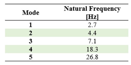
The vibration modes of the components were obtained to know their natural frequencies. These eigenmodes represent characteristic patterns of vibration of the system. For each eigenmode, a modal amplitude indicating the magnitude of vibration associated with that mode is determined. Modal amplitudes are important in modal analysis because they allow us to understand how vibration is distributed in the system and what are the predominant directions of motion. Table 6 shows the modes of vibration.
Random vibration analysis is used to evaluate deformations, stresses, or displacements, which are based on the normal distribution. This is characterized by being symmetrical and having a bell shape. Like the one shown in Figure 11.
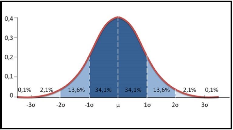
Fig. 11.
Gaussian bell.
It is defined [12] by two parameters: the mean, which determines the center of the distribution, and the standard deviation, which indicates the dispersion of the data around the mean. The standard deviation is denoted by σ, between -1σ to 1σ represent 68.2% of the data, between -2σ to 2σ 95.4% and between -3σ to 3σ 99.7%.
To obtain the equivalent stress the standard deviation value of 2 sigma was selected. This choice implies a probability of 95.45% that the deformation will reach that maximum value or lower. In addition, it allows the identification of the specific area of the component where this deformation would occur.
To find out if the material of the electrical harness bracket, the equivalent stress to which the part is subjected due to vibrations, does not exceed the elastic limit of the material and the maximum resistance to tension, Table 7 shows the mechanical properties of cold-rolled 1020 steel.
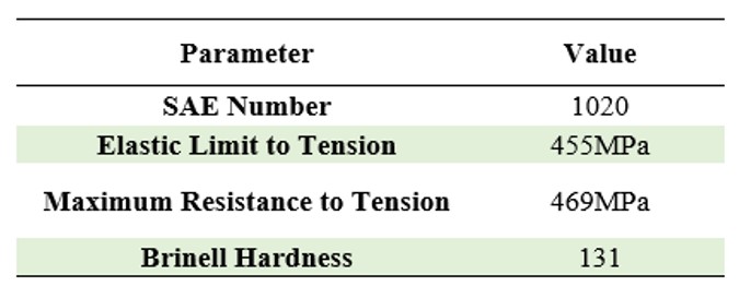
Once the yield strength of 455 MPa is reached, 1020 steel begins to undergo plastic deformation. This means that the deformation becomes permanent even after the applied stress is removed. In this region, the strain continues to increase with a relatively minor increase in stress.
As the stress increases further, a peak point called the maximum tensile strength is reached. At this point, the material gets its maximum strength and begins to weaken gradually.
After reaching maximum strength, the strain increases rapidly, and the material eventually fails at a point known as the fracture point. At this point, the deformation becomes uncontrollable, and the material breaks.
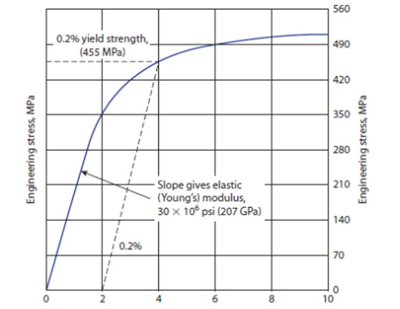
Fig. 12.
Stress-strain curve of 1020 steel.
According to the calculation of the equivalent stress carried out in ANSYS, the test that presented the highest comparable stress is the Highway test. In Figure 13, it is observed that the greatest equivalent stress is 1446.7 MPa. This value exceeds both the elastic limit of the material, which is 455 MPa and the maximum tensile strength of 469 MPa. The failure zone coincides with the actual fracture of the part. This information is important as it indicates that the component has experienced a significant load that has exceeded both its yield strength and ultimate strength.
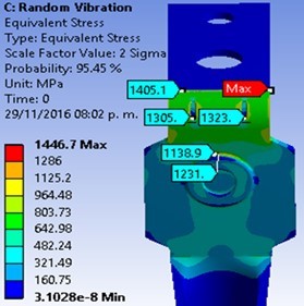
Fig. 13.
Equivalent stress calculation in ANSYS with data from the Highway test.
This implies that the component has undergone a permanent deformation and has reached a critical point of load that has led to its fracture. Equivalent stress analysis provides a detailed understanding of the component's load capacity and strength, which is essential for the design and evaluation of its performance under service conditions. Therefore, it is concluded that the Highway test has exerted excessive stress on the component, exceeding its resistance limits and causing its fracture. This information is valuable in identifying design weaknesses and taking corrective action to prevent future failures in similar applications.
VI. Conclusions
Based on the analysis carried out, it is concluded that the vibration mode with natural frequency 2 of the component coincides with the highest amplitude recorded in all the tests carried out in the frequency domain graphs, which is 4.4 Hz. This finding is significant, as it indicates that the component is experiencing a resonance effect at that specific frequency. Resonance occurs when the excitation frequency approaches or coincides with the natural frequency of vibration of the system. In this case, the coincidence between the natural frequency of vibration mode 2 and the highest amplitude in the graphs suggests that the component is being subjected to an excitation close to its resonant natural frequency. The resonance effect can have detrimental consequences, as it can amplify vibrations and stresses in the component, leading to fracture. The match between the resonant frequency and the maximum measured amplitude indicates that the component is experiencing high levels of vibration at that specific frequency, compromising its structural integrity.
Analysis of the frequency spectrum plots revealed that the spectrum density is concentrated between the frequencies of 1 and 12 Hz in all tests. This suggests that these frequencies are close to the natural frequency of the vehicle, which could be generating resonance and, therefore, the fracture of the part. Based on the deformation data, it can be concluded that the connector fails due to the vibrations to which it is subjected and fatigue in the arched area of the bent plate, aligning with the failure observed in the actual component.
To avoid damage, it is recommended to make modifications to the structural characteristics of the component. These modifications may include adjustments to its stiffness or mass, with the goal of altering its natural frequency. By performing calculations and simulations, it is possible to determine the necessary changes in component design or material to shift its natural frequency out of the excitation range.
In addition, other preventive measures can be considered, such as the addition of damping elements to dissipate vibrational energy and reduce the amplitude of vibrations. These elements can be damping materials or vibration-dissipating devices so that these frequencies do not affect the component.
In this project, the operation of the data acquisition system was also validated, which can be applied with other types of sensors to measure different magnitudes by changing the Arduino base program for the calibration of the sensor that needs to be added.
Referencias
[1] S. C. S. Jucá, P. C. M. Carvalho, F. T. Brito, "A low-cost concept for data acquisition systems applied to decentralized renewable energy plants," Sensors (Basel), vol. 11, no. 1, pp. 743-756, 2011.
[2] S. Lee, S. J. Nam, J. K. Lee, "Real-time data acquisition system and HMI for MES," J. Mech. Sci. Technol., vol. 26, no. 8, pp. 2381-2388, 2012.
[3] M. Ambrož, "Raspberry Pi as a low-cost data acquisition system for human-powered vehicles," Measurement (Lond.), vol. 100, pp. 7-18, 2017.
[4] F. J. Maseda, I. López, I. Martija, P. Alkorta, A. J. Garrido, I. Garrido, "Sensors data analysis in supervisory control and data acquisition (SCADA) systems to foresee failures with an undetermined origin," Sensors (Basel), vol. 21, no. 8, 2021.
[5] D. A. dos Santos, A. M. de Souza Soares, W. L. M. Tupinambá, "Development of a portable data acquisition system for extensometry," Exp. Tech., vol. 46, no. 4, pp. 723-730, 2022.
[6] H. Iseki, "An approximate deformation analysis and FEM analysis for the incremental bulging of sheet metal using a spherical roller," J. Mater. Process. Technol., vol. 111, no. 1-3, pp. 150-154, 2001.
[7] M. M. MacLaughlin, D. M. Doolin, "Review of validation of the discontinuous deformation analysis (DDA) method," Int. J. Numer. Anal. Methods Geomech., vol. 30, no. 4, pp. 271-305, 2006.
[8] J. H. Wu, "Seismic landslide simulations in discontinuous deformation analysis," Comput. Geotech., vol. 37, no. 5, pp. 594-601, 2010.
[9] H. Yang, X. Xu, I. Neumann, "An automatic finite element modelling for deformation analysis of composite structures," Compos. Struct., vol. 212, pp. 434-438, 2019.
[10] M. Kim, T. Y. Park, S. Hong, "Experimental determination of the plastic deformation and fracture behavior of polypropylene composites under various strain rates," Polym. Test., vol. 93, no. 107010, 2021.
[11] A. K. Chopra, Dynamics of Structures: Theory and Applications to Earthquake Engineering USA: Prentice Hall, 2012.
[12] J. L. Devore, Modern Mathematical Statistics with Applications, USA: Springer, 2012
Información adicional
redalyc-journal-id: 614