1 Introduction

Brantas watershed (Figure 1) covers an area of approximately 14,103 km², equivalent to 30% of the East Java Province area (~ 47,075.35 km²). The main river length of Brantas reaches 320 km (Kementerian 2010).

This watershed comprises 19 regencies (district) and cities areas. Brantas areas cover the administrative regency/city of Malang, Kediri, Blitar, Nganjuk, Batu, Blitar, Tulungangung, Trenggalek, Jombang, Mojokerto, Sidoardjo and Surabaya. Population in the Brantas watershed was around 16.2 million in 2010 (census) and around 16.9 million in 2015 (projection) (BPS 2014). About 30% of the East Java population has occupied the watershed land resources for residential use, agricultural, urban and city facilities, road network, tourism site, plantation, industry, and other social-cultural and economic activities. Brantas river network supply water for residential use, gearing the industry, electricity source, drainage, irrigating the agricultural field, and tourism activities (JICA 2019). About 60% of the agricultural product of the province comes from the Brantas tributaries. Major reservoirs or dams have been constructed on the Brantas tributaries, i.e., D1 (Sengguruh reservoir), D2 (Sutami), D3 (Lahor), D4 (Selorejo), D5 (Lodoyo), D6 (Wlingi), D7 (Wonrorejo), D8 (Waru Turi), D9 (Menturus), D10 (Gunungsari), D11 (Gubeng), and D12 (Jagir Dams) (Figure1).

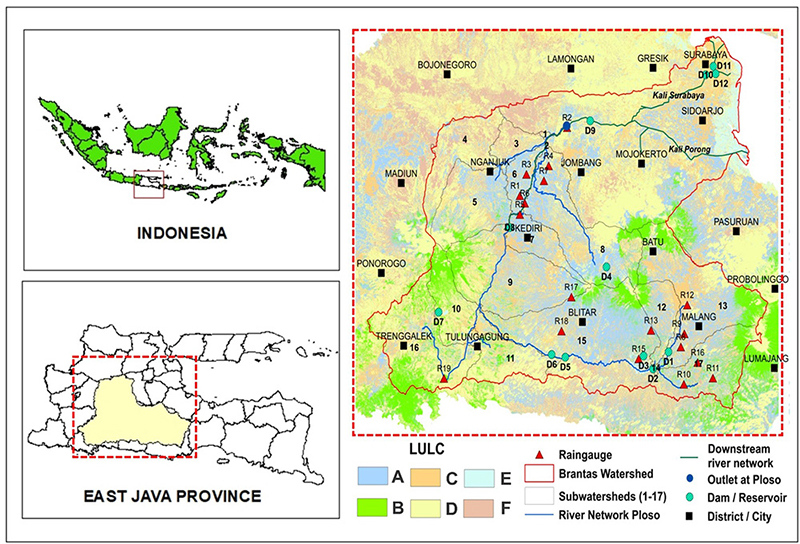
Figure 1
Study site with Land use and land cover: A. Irrigated paddy; B. Forest-Plantation; C. Settlement or pavement area; D. heterogeneous agricultural land; E. Shrubs land; F. Water Bodies.

Complexity of the watershed ecosystem requires a model to simplify the explanation of the watershed system. Soil & Water Assessment Tool (SWAT) models provide reliable features in analyzing this complex watershed. Several studies using SWAT models by (Joseph, Preetha & Narasimhan 2021; Liu et al. 2021; Rani and Sreekesh 2021) have succeeded in analyzing their watershed hydrological systems. Modeling this complex system of the watershed and using limited data available are challenging issues. Some questions arise, such as how to reduce the system’s complexity so that the essential hydrological processes are modeled? How to adjust the parameter’s value in the model with the limited data constraint? Thirdly, how to justify and explain that modelling processes and results can mimic the real phenomena questioned?

This study aims to analyze the SWAT model’s sensitive parameters using SWAT-CUP Tool and SUFI (Sequential Uncertainty Fitting) algorithm (Abbaspour 2015). Sensitivity analysis was conducted by following the previous publication (Arnold et al. 2012; Moreira, Schwamback & Rigo 2018; Brighenti et al. 2019). The hydrological processes are modeled at the monthly level. The sensitivity analysis operates at the monthly level. The study was conducted in Brantas Watershed in East Java Province, Indonesia.

The SWAT model (Krysanova & Arnold 2008) has more comprehensive equations and features. SWAT can calculate the discharge, erosion, sediment, and nutrient-related hydrological processes. The SWAT model uses the HRU (Hydrological Response Unit) concept to calculate spatially distributed hydrological processes (Arnold et al. 2012). The vertical components of water balance are calculated for each HRU. Then the runoff, sediment, and nutrient are accumulated from HRUs to each sub-basin. The horizontal movement of Water, nutrient, and sediment from each sub-basin to the watershed outlet is calculated using the transfers function (Arnold et al. 2012).

Many researchers around the world have used SWAT to study the impact of land use and land cover change, and climate change on hydrological processes, for example, the works by (Lamichhane & Shakya 2019) in Nepal (Spruce et al. 2018) in Mekong river basin (section: Thailand). A similar study was conducted by (Mireille et al. 2019) in Kenya.

2 Methodology

2.1 Input Data

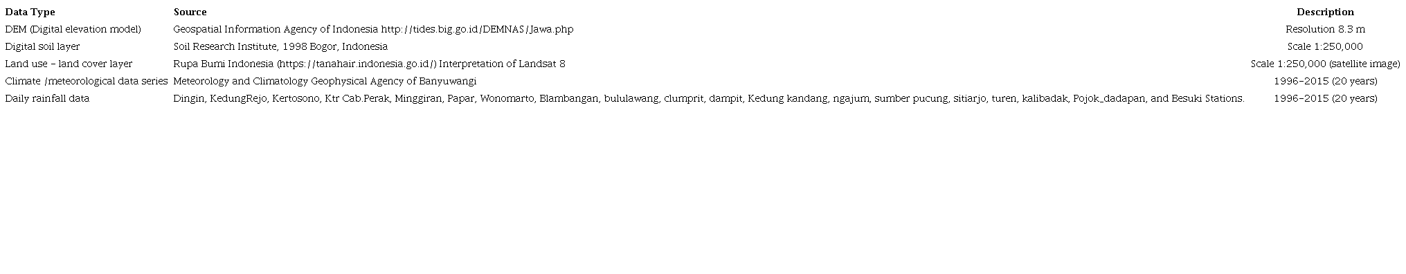
This study uses flow measurements located at Ploso. Then, from Ploso as an Outlet, the boundary of the sub-watershed is delineated. The sub-watershed area covers an area of 8,844.26 km² (Figure 1). The inputs for SWAT are the Digital Elevation Model (DEM), land cover, soil characteristics, climate variables (rainfall, temperature, solar radiation, relative wind speed, and humidity), and land management practice. All of the input data is necessary to be formatted in raster.

The DEM is derived from DEMNAS (BIG 2018). The DEMNAS is the DEM source at the National Scale provided by the Indonesian Agency of Geospatial Information or Badan Informasi Geospatial (BIG). The DEMNAS (BIG 2018) has a spatial resolution of 8.3 m x 8.3 m and is excellent for watershed delineation. In this case, the DEMNAS determines the sub-watershed boundary and derives the river network. Figure 2 visualizes the DEM, soil type layer, land cover in 2001, and land cover in 2015 of the Ploso sub-watershed. The altitude on the watershed varies from 17 to 3,653 m above sea level (Figure 2).

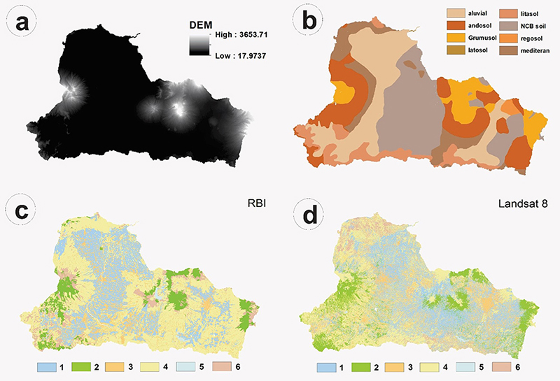
Figure 2
Input data: A. Altitude (m); B. Soil Type; C. Land cover (2001); D. Land cover (2015). 1. Irrigated paddy; 2. Forest-Plantation; 3. Settlement or pavement area; 4. Heterogeneous agriculture land; 5. Shrubs land; 6. Water Bodies.

Soil layer map is obtained from the national soil layer map database (Balitbang Pertanian 2014). The major soil type class on the watershed include: aluvial (24.5%), andosol (19.5%), grumosol (9.8%), latosol (0.02%), litosol (8.4%), regosol (10.4%), MCB soil (0.9%), mediteran (26.5%). The slope is derived from DEM. Slope classification follows the provisions of the Indonesian Ministry of Forestry, namely 0 - 8% (10.6%), 8 - 15% (26.1%), 15 - 25% (36.3%), 25 - 40% (15.7%), and > 40% (11.3%).

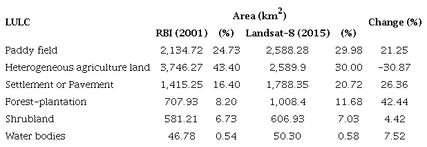
This study covers the period from 1996 to 2015. This study uses two editions of Land use (LU) and land Cover (LC) maps. The first map is a clip from the digital maps of RBI (Rupa Bumi Indonesia) (BIG 2018). The RBI map was produced during the year 2000-2001. The second map clip from the classified Landsat-8 Image. The available time series data were divided into periods 1 (1996-2005) and 2 (2006-2015). The model is run according to the period. The RBI represented the LULC for the first period. In comparison, Landsat represents the LULC for the second period (Figures 2C and 2D). LULC in Brantas from 2001 to 2015 experienced significant changes. The change is marked by increasing irrigated paddy fields (+21.24%) and forests-plantation areas (+42.44%). The land occupied for urban or pavement areas is also increased by +26.36% from the beginning. Contrary, the increase of LULC class above is compensated by the decrease in agricultural land (non-irrigated area) by -30.87% from the beginning (Table 1).

Table 1

LULC Change in Ploso sub-watershed.

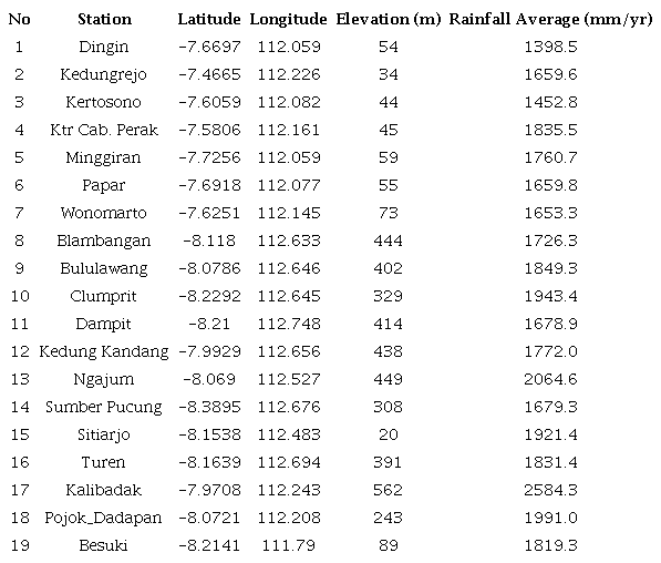
Rainfall data were obtained from 19 measurement sites (Table 2). The location of the rainfall measurement site is presented in Figure 1 (R1 to R19). The recording period for all the climate variables ranges from 1996 to 2015 (20 years). The discharge data is obtained from the existing AWLR (Automatic Water Level Recorder) located at the outlet of this watershed.

Table 2

Location of Rainfall Stations.

First, the discharge and rainfall data are obtained from the public offices of the water management and watershed authorities. The climate data (i.e., rainfall, temperature, solar radiation, wind speed, and humidity) were obtained from the nearby climatological stations. In this study, ArcSWAT 2012 is used as the primary tool for hydrological analysis, while GIS software aids visualization of the maps (Table 3).

Table 3

Description of model input.

2.2 Procedure

The general procedure of the modeling task consists of (1) watershed delineation and HRU determination, (2) writing table and climate data input, (3) creation of model output, and (4) calibration and validation. This step consists of sensitivity analysis and model performance evaluation for calibration and validation periods. The final step (5) is conducting the model simulation, water balance, and sediment yield analysis. Figure 3 presents the flowchart of the research procedure.

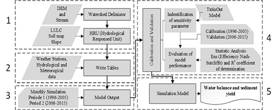
Figure 3
Flowchart of the modeling procedure.

2.2.1 Watershed delineation and HRU processing

In this case, the ArcSWAT module fills the sink to determine the flow direction and accumulation from the input DEM (DEMNAS). Then, the result uses to create the stream network, outlet, and sub-basin. The ArcSWAT will delineate the boundary of the watershed. Furthermore, the ArcSWAT produces HRUs (hydrological response units). HRU was constructed from three layers, overlay among land use (land cover), soil type, and slope classes. Finally, the HRU was determined using a 10% threshold.

2.2.2 Climate input (WritingTables)

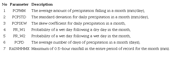
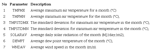
The SWAT-weather database (Weather Generator) use to calculate 14 necessary parameters. Seven (7) parameters depend on rainfall data (Table 4), and the other seven (7) parameters are adjusted for climate data (Table 5). Each parameter uses to update the SWAT database. The model will automatically calculate according to available data.

Table 4

The parameter is dependent on rainfall data.

Source: Arnold et al. (2012).

Table 5

Parameter determined from climate data.

Source: Arnold et al. (2012).

2.2.3 SWAT Output

Simulation results are read through the SWAT output menu. The model provides three types of output, i.e. (output.Rch: Flow_out) for calculated flow (in m3/s) and The “TxtInOut folder (output.std)” to visualize the calculated water balance result. Calibration is set for periods 1996 to 2005, and validation starts from 2006 to 2018 using flow data from the model. The SWAT GUI (graphical user interface) tests the model on the two periods.

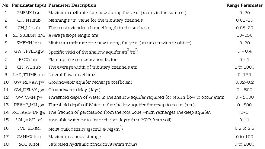
The SWAT CUP module was used to evaluate model performance. In this case, the SUFI-2 (Sequential Uncertainty Fitting) is explored to fit the parameter value during calibration and validation. Calibration and validation follow the procedure as published by Abbaspour (2015). Water balance is calculated at monthly and annual intervals. About 33 parameters are selected for sensitivity analysis by 500 iterations. Table 6 shows the 18 selected parameters. In this case, the r (multiples) and v (replace) procedures, as published by Abbaspour (2015), were used to find optimal parameter values.

Table 6

The estimated parameter value for calculating flow.

Source: Arnold et al. (2012).

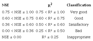
The model performance was evaluated by two statistical tests, i.e., Nash-Sutcliffe Efficiency (NSE) and determination coefficient (R2). Moriasi et al.(2007) stated that NSE values range between −∞ to 1, and NSE = 1 is the optimal value. NSE values between 0.0 and 1.0 are generally seen as an acceptable model performance, while NSE ≤ 0.0 indicates that model performance is unacceptable. The value of R² describes the correlation between observed and calculated (estimated) values. The higher value indicates a low error variant. R² = 0 shows no correlation between the observed and calculated values, whereas R² = 1 shows a strong correlation between observed and calculated values (Table 7).

Table 7

Classification of statistical indices.

Source: Moriasi et al. (2007).

Water balance and sediment yield are calculated during the simulation periods. The optimal parameter values are obtained from calibration, and validation is then used to run SWAT to calculate water balance and sediment yield at the location of interest.

3 Result and Discussion

3.1 Initial Calibration

Figure 4 shows the initial calibration result of SWAT to calculate flow at Ploso Outlet (Subbasin 1 in Model). The NSE and R² obtained are 0.05 and 0.01, respectively. Figure 4 indicates that the seasonal variation of a rainfall event is followed by seasonal variation in flow (discharge). Figure 4 also shows that the dot-line (calculated flow) starts from zero and increases linearly by a slope, which is unrelated to the observed flow and rainfall series. Therefore, it is necessary to search which parameters may be adjusted to mimic the observed flow and respond to the rainfall variation.

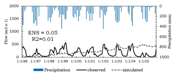
Figure 4
Initial calibration result for a period (Monthly 1996-2005).

3.2 Sensitivity Analysis

As listed in Table 6, parameter values are evaluated through iteration processes on the SWAT CUP module. Figure 5 shows the best-fitted result of parameter values. The “t-Stat” value (in Figure 5) indicates the sensitivity of the parameter. The zero (0) of the “t-Stat” value shows the most sensitive parameter. Furthermore, the “P-Value” visualizes how the strength of such a parameter contributes to the flow calculation. The “P-Value” close to one (1) signifier is the most determinant parameter. Therefore, the change in calculated flow is more significant by changing or manipulating this parameter’s value (Abbaspour 2015).

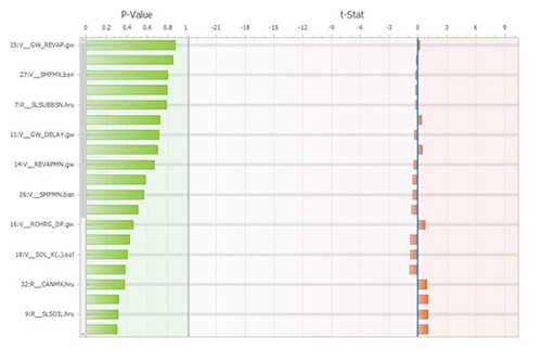
Figure 5
Sensitive parameters (Source: own SWAT CUP analysis).

As presented in Figure 5, the sensitivity result is obtained after 10x simulation processes and is treated with 500 iterations for each simulation. Finally, Table 8 presents the fitted 18 parameters that perform more sensitively to produce runoff for the Ploso sub-watershed. Nine parameters are more sensitive (>50% sensitivity) than others. These include (GW_REVAP, ESCO, SMFMX, SOL_AWC, SLSUBBSN, CH_N1, GW_DELAY, CH_L1, dan REVAPMN). Four parameters (ESCO, SOL-AWC, SOL_BD, and SOL_K) correlated to the soil layer’s runoff generation and water movement. Then, eight parameters (i.e., GW_REVAP, SMFMX, GW_DELAY, REVAPMN, SMFMN, GW_SPYLD, RCHRG_DP, and GWQMN) correlated to baseflow calculation (Brighenti et al. 2019).

Table 8

The fitted value of each parameter. The colored lines show the sensitive parameters having a value of more than > 50%, while non-colored lines show the fewer sensitive parameters.

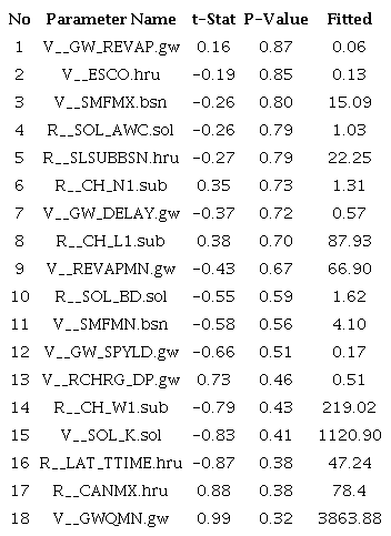
Other parameters, such as CH_N1, CH_L1, CH_W1, and LAT_TIME, influence the properties and flow velocity at the main river channel. Specific parameters related to the groundwater (gw) significantly influence the streamflow calculation. For example, the parameter “GW_REVAP.gw” is gradually modified from 0.02 to 0.06 to increase the baseflow level until the vegetation root zone is reached. The increasing value of “GW_REVAP.gw” normalized the calculation of potential evapotranspiration. The root zone will be saturated, then less or no water will infiltrate the soil and increase runoff production. Therefore, the REVAPMN parameter value should be reduced from 750 to 66.9 to increase Water until the root zone. In this case, the parameter “GW_REVAP.gw” has 87% sensitivity, and the REVAPMN parameter got 67% sensitivity.

Moreover, reducing the value of “GW_DELAY.gw” from 31 to 0.57 will accelerate the filling time of the aquifer zone. Furthermore, increasing the value of “GW_SPYLD.gw” from 0.003 to 0.27 did the balanced ratio between water volume and rock material in the unsaturated zone. The “GWQMN.gw” value increased from 1000 to 3863.88 to compensate for other groundwater parameters and reversely permit water flow in the unsaturated zone. The “RCHRG_DP” is adjusted from 0.05 to 0.51 to recharge the deep aquifer from the root zone through percolation.

Moreover, parameters describing soil properties are adjusted to maintain the water content f the soil layers at a certain level (for example, SOL_AWC from 0.11 to 1.03, SOL_BD from 1.1 to 1.62 SOL_K from 5.4 to 1120.90 ). Also, related parameters for describing HRU, Basin, and Sub-basin are optimized; for example, the ESCO value is set up from 0.95 to 0.13 to reduce the evaporation level. SL-SUBBSN is adjusted from 91.46 to 22.25; LAT_TTIME is increased from 0 to 47.24 (Table 8). Therefore, adjusting these parameters’ values increases the model performance in calculating flow.

3.3 Hydrograph Results

Figure 6 shows the observed and calculated hydrograph of monthly flow for calibration periods from 1996 to 2005. The calibration produces NSE = 0.66 and R² = 0.67. The calculated flow pattern is more adjusted and follows the fluctuation of observed flow and rainfall events.

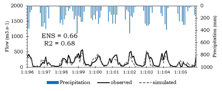
Figure 6
Hydrograph of monthly flow (for calibration periods 1996-2005).

Figure 7 shows the simulated and observed hydrograph of monthly flow during the validation periods from 2006 to 2015. The validation processes produce NSE and R² = 0.55 and 0.56, respectively.

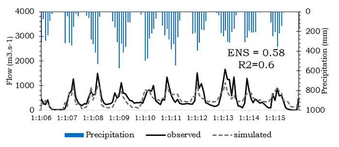
Figure 7
Hydrograph of monthly flow for the validation period (from 2006-2015).

3.4 Hydrological Simulation of the SWAT Model

Figure 8 illustrates an overview of the annual SWAT simulation. We can divide the result into three periods. The average annual rainfall series is divided into three segments (1^st red line = 3,009.9 mm/yr, 2^nd red line = 1,860.1 mm/yr, and 3^rd red line = 3,946.3 mm/yr). Similarly, we can divide the average annual sediment yield into three segments (1^st black line = 1,547.7 ton/ha/yr, 2^nd = 890.4 ton/ha/yr, and 3^rd = 3,600.0 ton/ha/yr). Finally, the average annual water yield was divided into three segments (first green line =2,481.8 mm/yr, second = 1,413.7 mm/yr, third = 3,522.0 mm/yr). The distribution of water yield and sediment follows the fluctuation of rainfall.

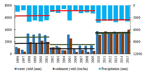
Figure 8
Resume of the SWAT Model Simulation.

The previous studies have reported that the abundance of rainfall in segment 3 ( from 2014 to 2015) caused flood events in four districts on the Brantas watershed (Erlina, 2018) and increased sediment concentration by 60.50%. The sediment deposit propagated by a flood event reduced the capacity of 6 large reservoirs (2005-2006) in the Brantas (Kementerian 2010).

4 Conclusion

Sensitivity analysis of the SWAT model using the SWAT-CUP tool with the SUFI-2 method affects the results of model adjustments. The calibration results increased ENS from 0.05 to 0.06 as well as R² from 0.01 to 0.68. The same as validation in the satisfactory category in Brantas watershed. The analysis show that 18 parameters are sensitives. The nine (9) parameters have a sensitivity level of 50% (GW_REVAP, ESCO, SMFMX, SOL_AWC, SLSUBBSN, CH_N1, GW_DELAY, CH_L1, and REVAPMN). The four parameters (ESCO, SOL-AWC, SOL_BD, and SOL_K) correlated to the soil layer’s runoff generation and water movement. Then, eight (8) parameters (GW_REVAP, SMFMX, GW_DELAY, REVAPMN, SMFMN, GW_SPYLD, RCHRG_DP, and GWQMN) correlated to baseflow calculation. The model simulation illustrates that rainfall and land cover changes drive the hydrological processes, producing more water yield and sediment in the Brantas watershed.

5 Acknowledgments

This article’s publication is supported by a Reworking “Skripsi” Grant from the Research Institute (LP2M), University of Jember, 2019 - 2020.

6 References

Abbaspour, K. 2015, 'SWAT-CUP Calibration and uncertainty programs', User Manual, pp. 1596-602, DOI:10.1007/s00402-009-1032-4.

Arnold, J.G., Moriasi, D.N., Gassman, P.W., Abbaspour, K.C., White, M.J., Srinivassan, R., Santhi, C., Harmel, R.D., van Griensven, A., Van Liew, M.W., Kannan, N. & Jha, M.K. 2012, 'Swat: model use, calibration, and validation', American Society of Agricultural and Biological Engineers, vol. 55, no. 4, pp. 1491-508.

Balitbang Pertanian 2014, Peta tanah dengan skala 1:50.000, Indonesian Agency for Agricultural Research and Development, viewed 12 January 2019, <http://balittanah.litbang.pertanian.go.id/ind/>.

BIG ‒ Badan Informasi Geospasial 2018, Seamless Digital Elevation Model (DEM) dan Batimetri Nasional, Badan Informasi Geospatial, viewed 12 January 2019, <http://tides.big.go.id/DEMNAS/>.

BPS ‒ Badan Pusat Statistik 2014, Proyeksi Penduduk Jawa Timur 2010 - 2020, Surabaya, viewed 12 January 2019, <https://jatim.bps.go.id>.

Brighenti, T.M., Bonumá, N.B., Grison, F., Mota, A.A., Kobiyama, M. & Chaffe, P.L.B. 2019, 'Two calibration methods for modeling streamflow and suspended sediment with the swat model', Ecological Engineering, vol. 127, pp. 103-13, DOI:10.1016/j.ecoleng.2018.11.007.

Erlina, E. 2018, 'Analisis Banjir Dan Sedimentasi Wilayah Sungai Brantas (Tinjaun Terhadap Metode Pengendalian)', Jurnal Teknik Sipil, vol. XIII, no. 1, pp. 1-14, DOI:10.47200/jts.v13i1.835.

JICA ‒ Japan International Cooperation Agency 2019, The Republic of Indonesia, the project for assessing and integrating climate change impacts into the water resources management plans for Brantas and Musi river basins: water resources management plan: final report, vol. II, Main Report, Japan, viewed 12 January 2019, <https://openjicareport.jica.go.jp/619/619/619_108_12353090.html>.

Joseph, N., Preetha, P.P. & Narasimhan, B. 2021, 'Assessment of environmental flow requirements using a coupled surface water-groundwater model and a flow health tool: A case study of Son river in the Ganga basin', Ecological Indicators, vol. 121, 107110, DOI: 10.1016/j.ecolind.2020.107110.

Kementerian, P.U.P.R. 2010, Pengelolaan sumber daya air wilayah sungai bengawan solo, Menteneri Pekeraan Umum Republik Indonesia, Jakarta.

Krysanova, V. & Arnold, J.G. 2008, 'Advances in ecohydrological modeling with SWAT-a review', Hydrological Sciences Journal, vol. 53, no. 5, pp. 939-47, DOI:10.1623/hysj.53.5.939.

Lamichhane, S. & Shakya, N.M. 2019, 'Integrated assessment of climate change and land use change impacts on hydrology in the Kathmandu Valley Watershed, Central Nepal', Water, vol. 11, no. 10, 2059, DOI: 10.3390/w11102059.

Liu, Z., Herman, J.D., Huang, G., Kadir, T. & Dahlke, H.E. 2021, 'Identifying climate change impacts on surface water supply in the southern Central Valley, California', Science of the Total Environment, vol. 759, 143429, DOI:10.1016/j.scitotenv.2020.143429.

Mireille, N.M., Mwangi, H.M., Mwangi, J.K. & Gathenya, J.M. 2019, 'Analysis of land use change and its impact on the hydrology of kakia and esamburmbur sub-watersheds of Narok County, Kenya', Hydrology, vol. 6, no. 4, 86, DOI:10.3390/hydrology6040086.

Moreira, L.L., Schwamback, D. & Rigo, D. 2018, 'Sensitivity analysis of the Soil and Water Assessment Tools (SWAT) model in streamflow modeling in a rural river basin', Revista Ambiente e Agua, vol. 13, no. 6, e2221, DOI:10.4136/ambi-agua.2221.

Moriasi, D.N., Arnold, J.G., Van Liew, M.W., Bingner, R.L., Harmel, R.D. & Veith, T.L. 2007, 'Model evaluation guidelines for systematic quantification of accuracy in watershed simulations', American Society of Agricultural and Biological Engineers, vol. 50, no. 3, pp. 885-900, DOI:10.13031/2013.23153.

Rani, S. & Sreekesh, S. 2021, 'Flow regime changes under future climate and land cover scenarios in the Upper Beas basin of Himalaya using SWAT model', International Journal of Environmental Studies, vol. 78, no. 3, pp. 382-97, DOI:10.1080/00207233.2020.1811574.

Spruce, J., Bolten, J., Srinivasan, R. & Lakshmi, V. 2018, 'Developing land use land cover maps for the lower mekong basin to aid hydrologic modeling and basin planning', Remote Sensing, vol. 10, no. 12, 1910, DOI:10.3390/rs10121910.

Data availability statement

Funding information

Author notes

E-mail: wawan201093@gmail.comE-mail: indarto.ftp@unej.ac.idE-mail: idamandala.faperta@unej.ac.id

Conflict of interest declaration