1 Introduction

In the recent readjustment of the High Precision Altimetric Network (RAAP - “Rede Altimétrica de Alta Precisão” in Portuguese) of the Brazilian Geodetic System (BGS), using geopotential numbers, a normal heights system has been adopted. According to IBGE (2019), this type of height has been adopted because it is the most suitable for modern scientific concepts and methods and is in line with the context of the International Association of Geodesy (IAG) to define the future International Height Reference System (IHRS).

In addition to adopting normal heights, the readjustment also took into account new observations of spirit leveling and gravimetry, and inconsistencies corrections. While the IHRS is not realized in Brazil, most normal heights remain referred to IBVD, and the smallest part, in the Amapá state, is referred to SBVD. These datums are of a local nature, since they were defined from Mean Sea Level (MSL) observed values in each region, using unique tide gauge stations (IBGE 2019).

In order to obtain normal height values ​​referred to IBVD or SBVD at a given point, using terrestrial methods, the transport of heights from the nearest benchmark (RN - “Referência de Nível” in Portuguese) station must use a spirit or trigonometric leveling. However, with the popularization of GNSS receivers in the last decades in Brazil and with the development of GGMs, from which it is possible to obtain a global quasi-geoid model, there is an alternative to the leveling process within a specific limit of accuracy. This alternative is more economical and requires less processing time. Mainly in places where the nearest RN is tens or hundreds of kilometers away, a reality in some regions in Brazil.

Using a GGM, it is possible to suppress part of the omission error in height anomalies with the use of the well-known and widely applied Residual Terrain Modeling technique (RTM; Forsberg & Tscherning 1981). It is a way to increase the spectral resolution of a GGM, where the gravitational attraction of the masses distributed along a residual topography is used. That is, between a detailed topographic surface obtained from a high-resolution Digital Terrain Model (DTM) and a smoothed topographic surface obtained from a low-resolution DTM in which the spectral information is considered to be already contained in the GGM (Heck & Seitz 2007; Hirt, Featherstone & Marti 2010; Gerlach & Rummel 2012; Grombein, Seitz & Heck 2017), the result is a refined GGM using DTMs.

The normal heights obtained by GNSS/GGM are referred to a global Vertical Reference System (VRS) associated with the GGM/RTM solution used. Thus, the reference surface for the calculated heights is not the same as defined by the MSLs obtained by tide gauges in IBVD and SBVD. Consequently, estimating transformation parameters between the different VRSs must consider a height datum offset. In addition, there is the issue of remaining omission errors concerning the full spectral information of the tide gauge solution.

The problem is not unique to Brazil. Researchers have proposed several approaches in several countries and regions around the world for more than three decades. Among them, some of the most widely used can be mentioned: the approach based on the mean of the discrepancies between height anomalies (Kasenda 2009; Grombein, Seitz & Heck 2017); the approach based on the zero-level geopotential values (Burša et al. 1999; De Freitas 2015; Sánchez, De Freitas & Barzaghi 2018; Ihde et al. 2017); and the approach based on the GBVP solution (Rummel & Teunissen 1988; Xu 1992; Gerlach & Rummel 2012; Amjadiparvar, Rangelova & Sideris 2016; Grombein, Seitz & Heck 2016; Zhang et al. 2020).

In Brazil, with the old RAAP normal orthometric heights, Ferreira, De Freitas and Heck (2016) analyzed the use of the approach based on parametric modeling for the entire national territory. Specifically for the São Paulo state, in the context of the new RAAP normal heights, Delgado and Rodrigues (2022) have investigated the use of the geopotential-based approach with an adaptation. In this, the zero-level geopotential value for the local case was calculated using an arithmetic mean of the height anomalies discrepancies.

However, an essential factor to be analyzed with the use of the approaches based on the mean of discrepancies between height anomalies, the GBPV solution, and the use of the zero-level geopotential value are the approximation and measurement errors in the input data set for the estimation of the transformation parameters (Kotsakis, Katsambalos & Ampatzidis 2012; Ferreira, De Freitas & Heck 2016). According to Grombein, Seitz and Heck (2017), these errors cause biases in the height datum offset, which will vary regionally. The authors also mention that for GNSS ellipsoidal heights and GGM-derived height anomalies are expected errors to be mainly random. On the other hand, the physical heights associated with the Local Vertical Datums (LVD) can additionally be affected by systematic leveling errors and distortions in the leveling network.

In order to minimize this problem, there are two ways: (i) estimation of local parameters, as in Delgado and Rodrigues (2022), or (ii) the use of the approach based on the use of parametric modeling as a function of geodetic coordinates (Kotsakis, Katsambalos & Ampatzidis 2012; Rülke et al. 2012; Grombein, Seitz & Heck 2017).

This paper analyzes the use of GNSS and XGM2019 GGM, refined with the RTM technique, to determine normal heights in two Brazilian regions, using the four different approaches mentioned for linkage to IBVD and SBVD. Approaches based on the mean of discrepancies between height anomalies, the use of the zero-level geopotential value and on the GBVP solution, adopt the idea of ​​local parameter estimation. Furthermore, the weighted mean of the height anomalies discrepancies has been used in the first two approaches, taking into account the input data uncertainties.

2 Methodology and Data

Considering the methodology used in this research, Figure 1 shows the step flow, from obtaining the data set to the step of evaluate the accuracy of the linkage performed using each approach.

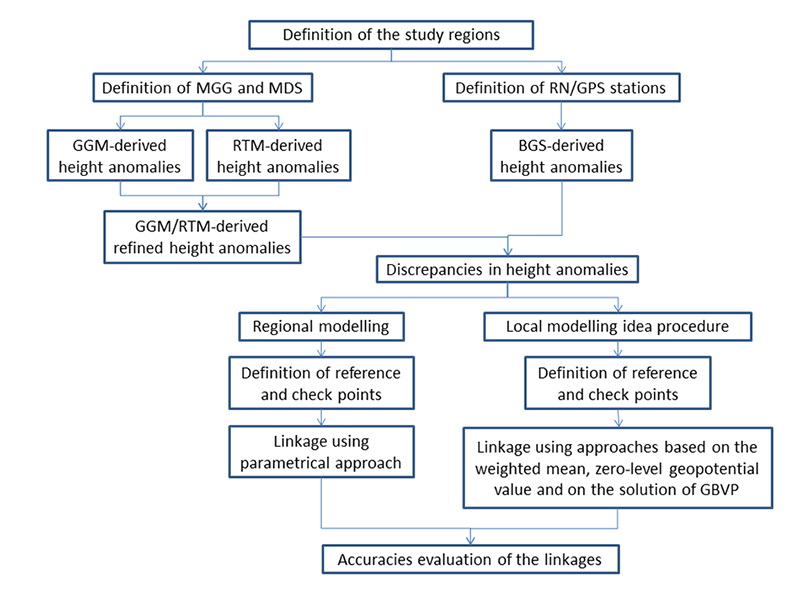
Figure 1
Principle of unification of HRS using zero-level geopotential values.

2.1 Approaches for Linking GNSS/GGM/RTM Normal Heights to Brazilian Vertical Datums

GNSS/GGM/RTM-derived normal heights are referenced to a VRS associated with a zero-level geopotential global value W₀ of the used GGM solution. Thus, for such global heights to be linked to any of the Brazilian Vertical Datums (BVDs), it is necessary to use some transformation approach. This section presents the approaches used in this research.

All used approaches require a set of n points with height anomaly values ​​associated with the BGS is required to estimate the parameters. These are the so-called RN/GPS connection stations, that is, connection stations between the RAAP and the BGS's GPS network. At these points, the subtraction of the ellipsoidal height referred to as the BGS by the normal height referred to one of the BVDs obtains the values ​​of height anomalies ζ_RN/GPS .

2.1.1 Approach Based on the Mean of the Height Anomalies Discrepancies

In the approach based on the mean of the height anomalies discrepancies, the transformation parameter to be applied at GNSS/GGM/RTM-derived normal heights values can be calculated by (Ferreira, De Freitas & Heck 2016) (Equation 1):

where ζ_{RN/GPS_i} and ζ_{GGM/RTM_i} are the height anomaly at a given station i associated with the BGS and the height anomaly at the same station i obtained from the GGM/RTM solution, respectively.

In this approach, the uncertainties of the input data influence the parameter estimation. This research, proposes, as a way of minimizing this influence, the propagation of the uncertainties associated with the GBS quantities when available. Thus, the weighted mean can be used, with weights inversely proportional to the square of the deviations. The height anomalies associated with the GGM/RTM solution are considered fixed and without error due to the absence of information. In this way, we have the Equations 2 and 3:

2.1.2 Approach Based on the Zero-level Geopotential Values

In the case of the approach based on zero-level geopotential values, the methodology presented by Ihde et al. (2017), adapted by Delgado and Rodrigues (2022), has been used. The objective is to obtain the zero-level geopotential value (W_0k ) of an LVD k. This quantity is the parameter to be estimated. Considering point P in Figure 2 as a BGS’s RN/GPS station, the anomalous potential at this point can be obtained from the GGM/RTM solution. On the other hand, the value of the ellipsoidal height h_P can be obtained free of charge from the BGS’s Geodetic Database.

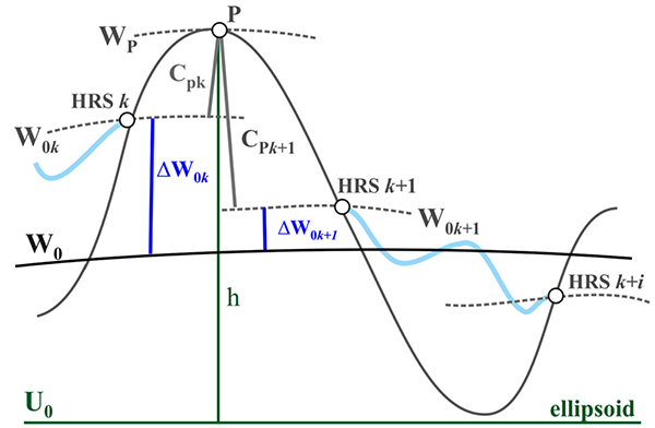
Figure 2
Principle of unification of HRS using zero-level geopotential values.
Source: Adapted from Ihde et al. (2017).

From the mathematical deduction presented in Delgado and Rodrigues (2022), with the W_0k,P values for the set of n points, the mean value of the potentials can be assumed as the local reference level (Equation 4):

where U₀ is the zero-level spheropotential value of the adopted Reference Ellipsoid (e.g., GRS80); and γ_i is the magnitude of the normal gravity acceleration at point i. Adopting the weighted mean with weights inversely proportional to the square of the propagated uncertainties of ζ_{i RN/GPS} we have the Equation 5:

Finally, to calculate the normal height obtained via GNSS/GGM/RTM at a given point Q, referred to the LVD k, we have the Equation 6:

2.1.3 Approach Based on the GBPV Solution

In the case of the approach based on the GBPV solution, proposed by Rummel and Teunissen (1988), not only the difference in zero-level geopotential but also the difference in terms of geopotential number is considered. In the adapted case of fixed GBVP solution, considering a LVD k, we have the Equation 7:

where ∆W₀ is the difference in zero-level geopotential; K(ψ)_i is the Hotine-Koch function at point i; and C_k = W₀ - W_0k . The ∆W₀ and C_k values are estimated as parameters in a least-squares adjustment. It is worth noting that the h_i and H^N_i,k values have uncertainties and were considered in the matrix of the weights of the observations in the adjustment.

2.1.4 Approach Based on the Parametric Modeling

As mentioned before, the approximation and measurements errors in the input dataset influence the estimation of parameters in the case of first three approaches presented in this. In order to take this problem into account, the idea of parametric modeling based on the use of polynomial functions of geodetic coordinates can be used. In this research, for the application of this approach, a plane functional mathematical modeling with three parameters and a scale factor have been used, as seen in Kotsakis et al. (2012) and Ferreira, De Freitas and Heck (2016) (Equation 8):

where δH^N_i0 , a_1, and a₂ are, respectively, the vertical offset between the vertical data, the tilt of the plane in the north-south and east-west direction, for the centroid (λ₀; φ₀) of the study region; δs is a scale factor that accounts for the potential correlation between the raw residuals and the topographic heights; λ_i and φ_i are the geodesic longitude and latitude at i-th point from 1 to n. To estimate δH^N_i0 , a₁, a_2, and δs values a Least-Squares adjustment has been used with weights in the observations as a function of the uncertainties of ζ_{i RN/GPS k} .

2.2 Local Parameters Estimation Idea

In order to consider the influences of approximation and measurement errors on the input data sets, ζ_{RN/GPS k} and ζ_GGM/RTM , the first three approaches used the idea of local parameters estimation, as in Delgado and Rodrigues (2022). That is, with more adjusted local modeling for the study regions from subsets of height anomalies data. Therefore, it could verify possible outliers in the set of discrepancy values ​​ζ_{P BGS} - ζ_{P GGM/RTM} before calculating the parameters. First, in the detection step, normality tests were performed with a 95% confidence level.

The normality tests have been used according to the sample size, providing greater detection accuracy: Shapiro-Wilk (Shapiro & Wilk 1965) for samples smaller than 50 observations and Jarque-Bera (Bera & Jarque 1980) for samples more significant than 50 observations. After performing the tests, the Data-Snooping method has been interactively applied to identify outliers to recognize one observation at a time, until the dataset is considered with a normal distribution and free of outliers.

After identifying outliers, the adaptation step verified the hypothesis of spatial correlation of outliers, that is, if the outliers have been spatially grouped in a subregion. Therefore, a spatial data clustering analysis technique has been used based on the standard deviation value, considering that spatially correlated outliers may indicate a different local bias from that verified in the rest of the data in the sample set, rather than simply the presence of gross error. Thus, using the first three approaches for the two study regions indicated in section 2.3, it was possible to carry out linkage studies for one or more areas, called study sub-regions, with different local parameters.

2.3 Study Regions, Data Collection and Validation of Linkage Approaches

For the development of this research, two study regions have been defined. The first region comprises the São Paulo state with 102 RN/GPS stations, as shown in Figure 3A. The second region is the Amapá state, with 67 RN/GPS stations, as shown in Figure 3B. While in the first region the normal heights are referred to the IBVD, in the second one the heights are referred to the SBVD.

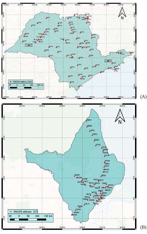
Figure 3
Study regions with the BGS RN/GPS stations spatial coverage: A. São Paulo; B. Amapá.

The estimation of the transformation parameters used 2/3 of the total number of available RN/GPS stations in each region, known as reference points (RP). The complementary part of 1/3 was used to assess the accuracy of the linkages, known as check points (CP). These amounts were empirically defined.

The GGM derived height anomaly values (ζ_{P GGM} ) were obtained from the ICGEM (International Center for Global Gravity Field Models) web interface for each station. This research used the GGM XGM2019 with maximum degrees and orders (XGM2019e_2159). This GGM was chosen considering its better accuracy in Brazilian territory than the other GGMs available (Zingerle, Pail & Gruber 2020).

To minimize the omission errors of the GGM data the RTM technique was used (Forsberg & Tscherning 1981). This technique considers the gravitational attraction of the residual topographical masses. Such data was extracted from DTMs, and the approach used was rectangular prisms with planar approximation (Heck & Seitz 2007), with a radius of 200 km, as used by Hirt, Featherstone and Marti (2010). For a given point P, after calculating the residual height anomaly, obtained by the RTM technique (ζ_{P RTM} ), the refinement of the height anomaly extracted from the GGM XGM2019 (ζ_{P GGM} ) can be done by Equation 9:

where ζ_{P GGM/RTM} is the height anomaly extracted from the GGM and refined by the RTM technique.

The selected DTMs had the best cost/benefit ratio based on factors such as accuracy, computational cost and resolution in previous tests performed by the authors. Therefore, it was chosen the ETOPO1 (Amante & Eakins 2009) model with 1’ spatial resolution and the SRTM15_PLUS (Tozer et al. 2019) 15” spatial resolution, obtained from the ICGEM and the ERDDAP data server of the National Oceanic and Atmospheric Administration (NOAA), respectively. The application of the RTM technique uses the ETOPO1 as reference smoothed surface and theSRTM15_PLUS model as detailed surface. Both models cover oceanic areas derived from bathymetric data.

Before the integrating of the data, it considered the differences in Permanent Tide Systems. To make the BGS’s ellipsoidal heights (tide free) compatible with the RAAP normal heights (mean tide) and GGM/RTM heights (zero tide), the transformation to the mean tide System has been defined using the formulation presented by Rapp (1989). This was recommended by the IAG, and presented in conventions for adopting of the IHRS (Ihde et al. 2017).

For the evaluation of the linkages in each third, the Root Mean Square Error (RMSE) values have been calculated from the discrepancy dataset between the normal height values at the t checkpoints by Equations 10 and 11:

with:

where H^N_{i,trf_BVD k} is the i-th normal height obtained via GNSS/GGM/RTM referred to one of the BVD k at a given checkpoint i; H^N_{i, BVD k} is the i-th normal reference height (RN) at checkpoint i; and t is the number of checkpoints.

4 Results

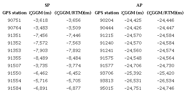
Table 1 shows an extract of the height anomalies ${\zeta }_{GGM/RTM}$ extracted from the GGM and refined by the RTM technique for the SP and AP study regions. As can be seen, at some stations, the RTM contribution reached values at the centimeter level. For example, the highest RTM height anomaly values have been 0.039 m at station 91634 in the SP region and 0.035 m at station 95068 in the AP region.

Table 1

Height anomalies in the SP and AP study regions (extract).

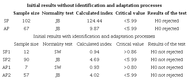
The normality hypothesis was not accepted in both regions, in the case of the first three approaches, after applying the normality tests to the sets of height anomalies discrepancies (Table 2). That is, no single systematic effect that can be modeled directly with a single set of parameters. Therefore, after rejecting the normality hypothesis, the Data-Snooping method has been iteratively applied to identify outliers until the datasets to be considered with a normal distribution and free of outliers. Table 2 presents, for each study region and sub-region sample size (number of points), the applied normality test (Jarque-Bera - JB or Shapiro-Wilk - SW), the calculated index in each test, the critical value for the statistical distribution (χ² with 2 degrees of freedom for JB) using 5% of significance level and results of the test (H0 rejected or not rejected).

Table 2

Results of the normality test in the study regions and sub-regions.

After identifying the stations whose height anomalies discrepancies have been considered as outliers, the adaptation step carried out the process of special correlation analysis by clustering. Figures 4A and 4B show these results. As can be seen, in the first study region, there was a spatial cluster of outliers in the southern part with 12 stations. These are in red in Figure 4A, in a coastal and mountain region and have been called SP1 sub-region. Thus, the rest of the study region has been called SP2 sub-region. After the groupings, it was verified the normality in both data sets for the sub-regions (Table 1). This result shows different systematic effects in the sub-regions, arising from approximation and measurement errors in the input data sets, ζ_{RN/GPS k} and ζ_GGM/RTM .

In the second study region, as seen in Figure 4B, there were three groups of points, two of which notably presented points with the lower and higher discrepancy in height anomalies. In red are the points with the slightest discrepancy, defining the study sub-region AP1, in a place further away from the coast and with higher heights than the other points. The points with the most significant discrepancy are shown in green, in a flatter region, defining the AP2 study sub-region. The third group, in yellow, did not present a spatial correlation and was composed of only three stations. Therefore, this group was disregarded.

Based on these results, for both study regions, when using the first three approaches, it is important to link the normal heights to the BVD separated into sub-regions, with an estimation of different local parameters.

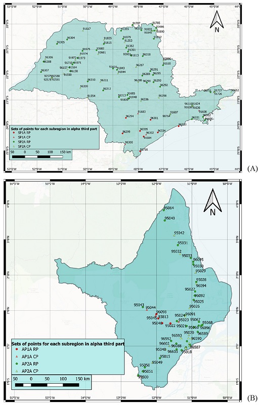
Figure 4
Clustering classification of points: A. in the first study region; B. in the second study region.

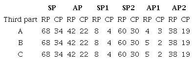
Three sets of these points have been tested to analyze differences in parameter estimation from different sets of RPs. Thus, an initial point configuration was called the Alpha third part (A). Subsequently, two other thirds, called Bravo (B) and Charlie (C) third parts have been defined, using permutations between the points. Table 3 shows the number of stations for each set of RP and CP.

Figures 4A and 4B show the distribution of RP and CP in all sub-regions using the Alpha third part as an example. The CPs in sub-regions SP1 and AP1 are indicated as triangles in faded red. The CPs in sub-regions SP2 and AP2 are indicated as triangles in light green.

Table 3

Number of stations for each set of RPs and CPs using third parts A, B and C.

After defining the sub-regions, in the first three approaches, the parameters and their uncertainties have been estimated with the three configurations of reference points A, B, and C. The first three approaches have not been used in the study regions due to the reasons explained in section 1. This is related to approximation and measurement errors in the input data set (systematic leveling errors and distortions in the leveling network) that generate different systematic effects in the height datum offset (Kotsakis, Katsambalos & Ampatzidis 2012; Ferreira, De Freitas & Heck 2016). According to Grombein, Seitz and Heck (2017).

For the case of the parametric modeling approach, the parameters have been estimated without dividing the study regions into sub-regions, for the reasons explained in section 2.1.4. Table 4 shows the results.

In the case of the SP1 and AP1 sub-regions, even with few points, the swap in the RPs has been adopted to fulfill the objective of analyzing differences in the estimated parameters with each third party. Table 4 shows that, in the case of the SP1 sub-region, the differences have been more significant than in the AP1 sub-region.

Table 4

Estimated parameters in the four approaches.

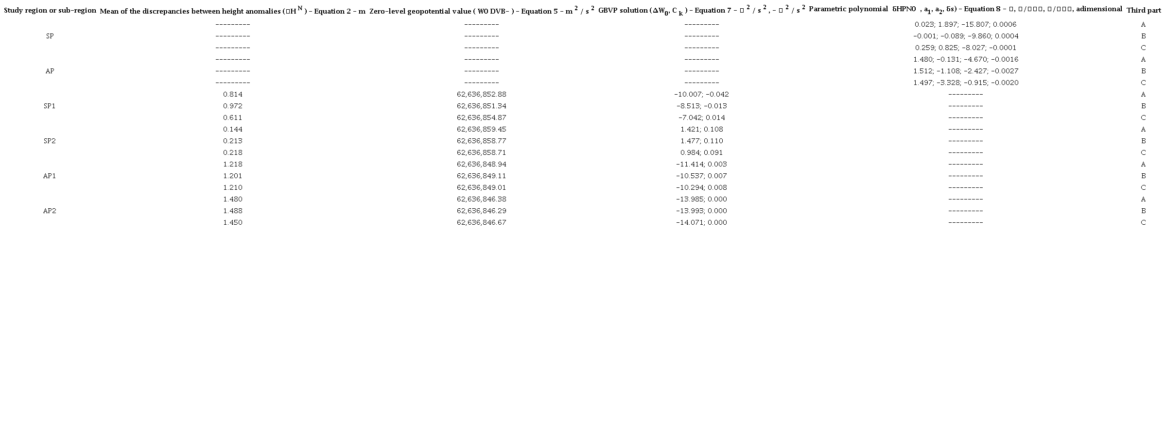
In the case of the approach based on the mean of the discrepancies between height anomalies, the parameters for the SP2 sub-region have been concordant at the millimeter level between the third parts B and C. Concerning the third part A, the difference has been almost 0.075 m. For the SP1 sub-region, the differences in the values ​​of the estimated parameters have been at the decimeter level with a maximum difference of 0.361 m between the third parts B, and C. In this case, the reduced samples of RPs may have influenced the disregard of some point or set of points that has contributed to the values ​​obtained in third parts A and B. For sub-region AP1, the most significant difference has been 0.017 m between thirds A and B. Among the other third parts, the difference has been at the level of a millimeter. For the AP2 sub-region, there was a difference at the millimeter level between the A and B thirds. In the case of the third part C, the differences to the other third parts have reached the centimeter level.

It is possible to analyze meter discrepancies using the approach based on the zero-level geopotential value by dividing the potential values by the mean normal gravity of the sub-region. In this case, the same differences obtained using the approach based on the mean of the discrepancies between height anomalies have been verified.

In the case of the approach based on the solution of the GBVP, the same procedure of dividing the parameters by the mean normal gravity of the sub-region has been performed. Regarding the parameter ∆W₀, in the SP1 sub-region, the differences reached the decimeter level, as in the case of using the previous approaches. The maximum difference has been approximately 0.300 m between third parts A and C. The difference between third parts B and C decreased by more than half compared to the previous approaches. For the SP2 sub-region, the difference between the third parts A and B has been approximately 0.006 m, which is ten times less than the result obtained from previous approaches. However, the other third parts’ differences have been at the level of the centimeter. In the AP1 sub-region, the differences have reached the centimeter level, with a maximum difference of approximately 0.110 m between the third parts A and C, which is almost ten times more than the difference obtained using the previous approaches. In the case of the AP2 sub-region, the differences have been all at the millimeter level. In the case of the parameter C_k , the differences have all been at the millimeter or sub millimeter level, with a maximum difference of approximately 0.006 m between the third parts A and C, in the SP1 sub-region. In the case of the AP2 sub-region, the values ​​of this parameter have been equal to zero, indicating that it is not significant.

In the case of the parametric modeling approach, the differences in the parameter δH^N_P0 between the third parts have been at decimeter level in the SP region and centimeter-level in the AP region. This may be related to a more significant variation of error values in the input data for the estimates since there are more points in the SP region. Regarding the plane tilt parameters in the north-south (a₂) and east-west (a₁) directions, the differences in rad have been more significant since they are dependent on the input geodetic coordinates differences. In the case of the scale factor, the values have agreed at the level of 10^-4 and 10^-3, for the SP and AP regions, respectively.

Given these results, it is possible to verify that there was no pattern in the differences between the parameters obtained with the third parts from one approach to another, except between the first and second approaches, whose results have been practically the same. Furthermore, differences can reach the decimeter level, even in the case of local modeling. However, except for the SP1 and AP1 sub-regions, the accuracy obtained using a given approach has remained practically the same, regardless of the third part used.

In the approach based on the zero-level geopotential value, it is possible to compare the estimated BVD zero-level geopotential values in the sub-regions with the values estimated in Sánchez & Sideris (2017), which used the entire RN/GPS stations networks in Brazil referred to IBVD and SBVD (Table 5). In Figures 5A and 5B are shown the differences in meters. The mean normal gravity values of the sub-regions were used to transform potential differences into metric differences. As can be seen, in some cases the difference can reach the decimeter level, which corroborates the hypothesis of estimating local parameters.

Table 5

Zero-level geopotential values obtained by Sánchez & Sideris (2017).

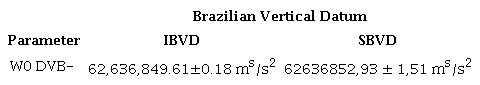
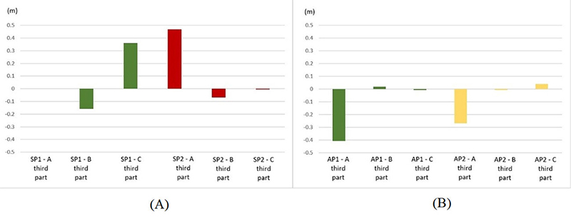
Figure 5
Differences of zero-level geopotentials values for Sánchez and Sideris (2017): A. SP1, SP2; B. AP1, AP2. Values level in meters.

After estimating the parameter, the accuracies of the linkages were calculated using the checkpoints in each study sub-region and third part, according to Equation 10. Figures 6 and 7 show the results. Here, the approaches based on the weighted mean of discrepancies between height anomalies, the zero-level geopotential value, the solution of the GBVP and the use of parametric modeling are called 1, 2, 3, and 4, respectively.

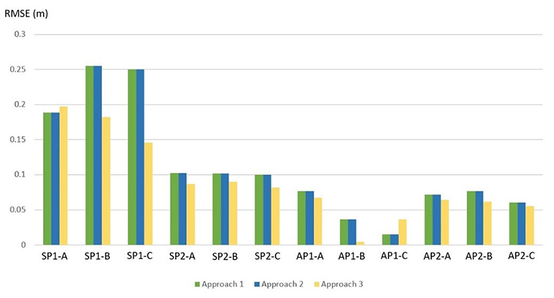
Figure 6
RMSE values of the discrepancies between HNi,trf_BVD k and HNi, BVD k in meters using approaches 1, 2 and 3.

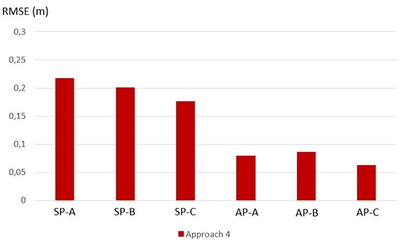
Figure 7
RMSE values of the discrepancies between HNi,trf_BVD k and HNi,BVD k in meters using approach 4

The RMSE values ​​for linkages using approaches 1 and 2 in all sub-regions and third parts have agreed at the sub-millimeter level. This indicates that the two approaches lead to similar results practically. Regarding approach 3, except for the SP1 sub-region/A third part and AP1 sub-region/ C third part, more accurate results have been found for the first two approaches. The results in the cases of exceptions can be related to the input data uncertainty levels at reference points, the model’s sensitivity in this regard, the distribution of the reference points, or even the low sampling for the parameter estimates. This is noticeable from the analysis of the difference between the results in the AP1 sub-region with the B and C third parts.

Using approaches with local parameters estimates in at least one of the sub-regions verifies less accurate values in the case of approach 4. The most significant differences in terms of RMSE reached decimeter levels. This result indicates that the parametric modeling, with an inclined plane in the north-south and east-west directions, considering a scale factor, has not been adequate for the transformation, considering the different local systematic effects present in the study regions.

In the SP1 and AP1 sub-regions, the permutations influenced the results regarding the choice of third parts of reference points. This can be related to the low sampling of the reference points and/or differences in error levels in the input data.

As can also be seen, in the SP1 sub-region, the results have been the least accurate, which may be related to the remaining omission errors or inaccuracies of the GGM/RTM solution. It should be noted that this sub-region is located in a mountainous area.

In terms of absolute values by sub-regions, it is observed that in the study region in São Paulo, the RMSE values have been higher. This could be related to three possible causes: the higher level of uncertainty at normal altitudes in the São Paulo region due to the propagation of errors in the leveling since the IBVD; the size of the areas; it is related to sampling. In the case of the state of Amapá, the RAAP is composed of only two relatively short leveling lines from the SVBD, which proposes a reduced and localized sample for calculating parameters. In addition, as the CPs are in this region, the results tend to be smaller. Consequently, in the regions of the state that are far from the sample, the parameters may not be adequate, and the accuracies may be worse.

5 Conclusion

This work evaluated the use of four approaches for linking normal altitudes obtained via GNSS/GGM refined by the RTM technique to the IBVD and SBVD Vertical Data. In the case of local modeling, after analyzing the spatial correlation of the outliers detected in each study region, it has been verified that they are spatially clustered. Thus, two sub-regions were defined in each of the study regions. Furthermore, it indicates the presence of different systematic effects in the sub-regions arising from approximation and measurement errors in the input data sets.

All tests used three different configurations of reference and checkpoint. The linkage accuracies have been calculated with the discrepancies in terms of normal heights at the checkpoints. In this context, it was possible to verify that the approaches based on the mean of the discrepancies between height anomalies and using the zero-level geopotential propose practically the same accuracy results. On the other hand, the approach based on the GBVP solution proposed better accuracy results concerning the first two approaches, except in two tests. The accuracy results have generally been worse compared to approaches with local modeling when using the approach based on parametric modeling.

For the here analyzed study regions, the linkages using the approach based on the GBVP solution with local modeling have generally been more accurate. However, considering the two exceptions, it is essential to check alternatively the use of the approach based on the mean of discrepancies between height, which is the simplest. The best results with the approach based on the GBVP solution may be related to the physical context of the modeling, which uses the zero-level geopotential difference, the geopotential number in the LVD and the coordinates of the reference points within the Hotine-Koch function. In addition, it is possible to affirm that there was a better fit of the data in the case of local modeling in the linkage.

This research’s results open up the prospect of obtaining normal altitudes via refined GNSS/GGM linked to BVD, replacing the transport of normal heights via leveling within a certain accuracy limit.

6 References

Amante, C. & Eakins, B.W. 2009, ETOPO1 1 Arc-Minute Global Relief Model: Procedures, Data Sources and Analysis, NOAA Technical Memorandum NESDIS NGDC-24, Colorado, viewed 25 March 2021, < 2009, ETOPO1 1 Arc-Minute Global Relief Model: Procedures, Data Sources and Analysis, NOAA Technical Memorandum NESDIS NGDC-24, Colorado, viewed 25 March 2021, https://ngdc.noaa.gov/mgg/global/relief/ETOPO1/docs/ETOPO1.pdf>.

Amjadiparvar, B., Rangelova, E. & Sideris, M.G. 2016, 'The GBVP approach for vertical datum unification: recent results in North America', Journal of Geodesy vol. 90, no. 1, pp. 45-63, DOI:10.1007/s00190-015-0855-8

Bera, A.; Jarque, C. 1980, 'Efficient test for normality, heterocedasticity and serial independence of regression residuals'. Econometrics Letters, vol. 6, pp. 255-259.

Burša, M., Kouba, J., Raděj, K., True, S.A., Vatrt, V. & Vojtíšková, M. 1999, 'Determination of the geopotential at the tide gauge defining the North American Vertical Datum 1988 (NAVD88)', Geomatica, vol. 53, pp. 459−66.

De Freitas, S.R.C. 2015, 'SIRGAS-WGIII activities for unifying height systems in Latin America', Revista Cartográfica. Pan-American Institute of Geography and History, vol. 91, no. 1, p. 75-92.

Delgado, R.E. & Rodrigues, T.L. 2022, 'Use of GNSS and a refined GGM (XGM2019e) for determining normal heights in the Imbituba Brazilian Vertical Datum and International Height Reference System', Bulletin of Geodetic Sciences, vol. 28, no. 2, e2022009, DOI:10.1590/s1982-21702022000200009

Ferreira, V.G., De Freitas, S.R.C. & Heck, B. 2016, 'Analysis of the discrepancy between the Brazilian vertical reference frame and GOCE-based geopotential models', in C. Rizos & P. Willis (eds), IAG 150 years, International Association of Geodesy Symposia, Springer, Berlin, pp. 227-32.

Forsberg, R. & Tscherning, C.C. 1981, 'The Use of Height Data in Gravity Field Approximation by Collocation', Journal of Geophysical Research, vol. 86, no. B9, pp. 7843-54, DOI:10.1029/JB086iB09p07843

Gerlach, C. & Rummel, R. 2012, 'Global height system unification with GOCE: a simulation study on the indirect bias term in the GBVP approach', Journal of Geodesy, vol. 87, no. 1, pp. 57-67, DOI:10.1007/s00190-012-0579-y

Grombein, T., Seitz, K. & Heck, B. 2016, 'Height system unification based on the fixed GBVP approach', in C. Rizos & P. Willis (eds), IAG 150 years, International Association of Geodesy Symposia, Springer, Berlin, pp. 305-11.

Grombein, T., Seitz, K. & Heck, B. 2017, 'On High‐Frequency Topography‐Implied Gravity Signals for a Height System Unification Using GOCE‐Based Global Geopotential Models', Surveys in Geophysics, vol. 38, no. 2, pp. 443‐77, DOI:10.1007/s10712-016-9400-4

Heck, B. & Seitz, K. 2007, 'A comparison of the tesseroid, prism and point-mass approaches for mass reductions in gravity field modelling', Journal of Geodesy, vol 81, pp. 121-36, DOI:10.1007/s00190-006-0094-0

Hirt, C., Featherstone, W.E. & Marti, U. 2010, 'Combining EGM2008 and SRTM/DTM2006.0 residual terrain model data to improve quasi-geoid computations in mountainous areas devoid of gravity data', Journal of Geodesy, vol 84, pp. 557-67, DOI:10.1007/s00190-010-0395-1

IBGE - Instituto Brasileiro de Geografia e Estatística 2019, Reajustamento da rede altimétrica com números geopotenciais, 2nd edn, IBGE, Coordenação de Geodésia, Diretoria de Geociências, Rio de Janeiro.

Ihde, J., Sánchez, L., Barzaghi, R., Drewes, H., Foerste, C., Gruber, T., Liebsch, G., Marti, U., Pail, R. & Sideris, M. 2017, 'Definition and Proposed Realization of the International Height Reference System (IHRS)', Surveys in Geophysics, vol. 38, no. 3, pp. 549-70, DOI:10.1007/s10712-017-9409-3

Kasenda, A. 2009, 'High precision geoid for modernization of height system in Indonesia', PhD dissertation, University of New South Wales.

Kotsakis, C., Katsambalos, K. & Ampatzidis, D. 2012, 'Estimation of the zero-height geopotential level W0 LVD in a local vertical datum from inversion of co-located GPS, leveling and geoid heights: a case study in the Hellenic islands', Journal of Geodesy, vol. 86, no. 6, pp. 423-39, DOI:10.1007/s00190-011-0530-7

Rapp, R.H. 1989, 'The treatment of permanent tidal effects in the analysis of satellite altimeter data for sea surface topography', Manuscripta Geodaetica, vol. 14, no. 6, pp. 368-72.

Rülke, A., Liebsch, G., Sacher, M., Schaëfer, U., Schirmer, U. & Ihde, J. 2012, 'Unification of European height system realizations', Journal of Geodetic Science, vol. 2, no. 4, pp. 343-54, DOI:10.2478/v10156-011-0048-1

Rummel, R. & Teunissen, P. 1988, 'Height datum definition, height datum connection and the role of the geodetic boundary value problem', Journal of Geodesy, vol. 62, pp. 477-98, DOI:10.1007/BF02520239

Sánchez, L. & Sideris, M.G. 2017, 'Vertical datum unification for the International Height Reference System (IHRS)', Geophysical Journal International, vol. 209, no. 2, pp. 570-86, DOI:10.1093/gji/ggx025

Sánchez, J.L.C., De Freitas, S.R.C. & Barzaghi, R. 2018, 'Offset Evaluation of the Ecuadorian Vertical Datum Related to the IHRS', Bulletin of Geodetic Sciences, vol. 24, no. 4, pp. 503-24, DOI:10.1590/s1982-21702018000400031

Shapiro, S. S.; Wilk, M. B. 1965, 'An Analysis of Variance Test for Normality (Complete Samples)', Biometrika Trust, vol. 52, pp. 591-609.

Tozer, B., Sandwell, D.T., Smith, W.H.F., Olson, C., Beale, J.R. & Wessel, P. 2019, 'Global Bathymetry and Topography at 15 Arc Sec: SRTM15+', Earth and Space Science, vol. 6, no. 10, pp. 1847-64, DOI:10.1029/2019EA000658

Xu, P. 1992, 'A quality investigation of global vertical datum connection', Geophysical Journal International, vol. 110, no. 2, pp. 361-70, DOI:10.1111/j.1365-246X.1992.tb00880.x

Zhang, P., Bao, L., Guo, D., Wu, L., Li, Q., Liu, H., Xue, Z. & Li, Z. 2020, 'Estimation of Vertical Datum Parameters Using the GBVP Approach Based on the Combined Global Geopotential Models', Remote Sensing, vol. 12, no. 24, e4137, DOI:10.3390/rs12244137

Zingerle, P., Pail, R. & Gruber, T. 2020, 'The combined global gravity field model XGM2019e', Journal of Geodesy, vol. 94, no. 66, pp. 1-12, DOI:10.1007/s00190-020-01398-0

Funding information

Data availability statement

Author notes

E-mail:rodrigoedelgado@gmail.comE-mail: tiagorodrigues@ufpr.br

Conflict of interest declaration