Article
Cut-cell Eta Model: History and Challenges Overcome
O Modelo Eta: História e Desafios Superados
 Fedor Mesinger fedor.mesinger@gmail.com
Cut-cell Eta Model: History and Challenges Overcome
Anuário do Instituto de Geociências, vol. 46, 56300, 2023
Universidade Federal do Rio de Janeiro
Received: 30 December 2022
Accepted: 10 April 2023
Abstract: Incentive for writing a limited area weather prediction model stemmed from the author's several years stay at the University of California in Los Angeles, at the end of the sixties. Exposed to what he refers to as the Akio Arakawa approach, having had an idea for a scheme that was an improvement to what Arakawa was using, and being aware of the importance of topography for the weather of the country he was to continue his career in, led in 1973 to his first limited area 3D code, the forerunner of what was to become the Eta model. Refinements and enhancements introduced by the author in subsequent years and of the collaborator he acquired, Zaviša Janjić, resulted in the code that when installed at the then U.S. National Meteorological Center, attracted attention. Hallmarks of the model were Mesinger's eta vertical coordinate, and Janjić's transformation of the Arakawa horizontal advection scheme to the model's semi-staggered B/E grid. In 1993 the Eta became the primary regional forecasting model of the U.S. Weather Bureau, and in 1998 its precipitation accuracy of 24-48 h forecasts became higher across all intensity thresholds than that of its predecessor, the Nested Grid Model (NGM) for its 00-24 h forecasts. Lately, the Eta is extensively used also as a regional climate model (RCM), mostly over the South American domain, and in near-real time as a tool for the North American Regional Reanalysis (NARR), run by the U.S. National Centers for Environmental Prediction/Climate Prediction Center. Several later unique numerical refinements of the Eta addressing problems noticed are summarized in a “before and after” fashion, and results are mentioned of its ensemble skill compared to that of its highly acclaimed driver European Centre for Medium-Range Weather Forecasts (ECMWF) model.
Keywords: Cut-cell schemes, Finite-volume schemes, Topography representation.
Resumo: O incentivo para escrever um modelo de previsão do tempo de área limitada resultou na estadia de vários anos do autor na Universidade da Califórnia, em Los Angeles, no final dos anos sessenta. Exposto ao que ele se refere como a abordagem de Akio Arakawa, tendo tido uma ideia para um esquema que era uma melhoria para o que Arakawa estava usando, e estando ciente da importância da topografia para o clima do país em que ele continuaria sua carreira, levou em 1973 ao seu primeiro código 3D de área limitada, o precursor do que viria a ser o modelo Eta. Refinamentos e aprimoramentos introduzidos pelo autor nos anos subsequentes e de seu colaborador, Zaviša Janjić, resultaram no código que, quando instalado no então Centro Meteorológico Nacional dos EUA, atraiu a atenção. As marcas registradas do modelo foram a coordenada vertical eta de Mesinger e a transformação de Janjić do esquema de advecção horizontal Arakawa para a grade B/E semi-escalonada do modelo. Em 1993, o Eta tornou-se o principal modelo de previsão regional do U.S. Weather Bureau e, em 1998, sua precisão de previsões de precipitação de 24-48 h tornou-se maior em todos os limiares de intensidade do que a de seu antecessor, o Nested Grid Model para suas previsões de 00-24 h. Ultimamente, o Eta é amplamente utilizado também como um modelo climático regional, principalmente sobre o domínio sul-americano, e em tempo quase real como uma ferramenta para a Reanálise Regional Norte-Americana, administrada pelo U.S. National Centers for Environmental Prediction/Climate Prediction Center. Vários refinamentos numéricos únicos posteriores do Eta abordando problemas detectados são resumidos de uma forma "antes e depois", e os resultados da habilidade da previsão por conjunto são expostos em comparação com o altamente aclamado modelo do European Centre for Medium-Range Weather Forecasts (ECMWF).
Palavras-chave: Esquemas de células cortadas, Esquemas de volumes finitos, Representação topográfica.
1 Introduction
A presentation of this type presumably is intended to acquaint people of sciences other than that of the presenter, to the extent possible, of what the efforts in the presenter's science are like. Be that as it may, this is what I will try to do. When enrolling to study meteorology I made my choice having a hard time deciding to abandon mathematics, physics, or chemistry, by choosing either one of those. It turned out that the first two years my curriculum consisted essentially just of the first two of those, no chemistry.
This was fine with me, weather processes being governed by the equations of motion, progress had to be based on a mathematical approach. With analyses of weather maps, then the only way of weather forecasting, I had problems. Marjan Čadež, the first person in Belgrade making efforts to contribute to atmospheric science using mathematics, had ideas of his own, not in agreement with the emerging possibilities of solving atmospheric equations, in some form, to help in predicting the weather. Programmable electronic computers in Belgrade at the time did not exist.
It was obvious to me that to join the developments of that kind I needed to be some time at a place where these developments were happening or at least followed. A good start was half a year on a project led by Friedrich Wippermann, at the Technical High School of Darmstadt. Eventually, at the end of the sixties, I ended up spending about three years at the best place possible for exposure to the emerging developments in atmospheric numerical modeling, at the University of California at Los Angeles (UCLA). This because of the ability to listen to the numerical methods course of Akio Arakawa.
Why would listening to a numerical methods course of an atmospheric sciences person, Arakawa, be more useful than studying one of the highly respected mathematics texts on difference methods of solving hyperbolic equations, or, initial value problems, such as, e.g., ( Richtmyer & Morton 1967)? While both such texts and atmospheric models deal with values of variables specified at grid points, the difference is in what these values represent. In mathematics texts, these are values of variables at the grid points. In atmospheric models, initial values at the grid points are derived from observations of various kinds. Better yet, they derive from “first guess” fields, modified based on observations. What they are considered to represent, depends on the so-called “dynamical core” of the model, schemes chosen for the terms of the equations of motion. In many, perhaps most dynamical cores, grid point values are considered to represent averages over the mass of air inside the grid cell of the model.
With grid point values valid across the volume of the grid cell, discontinuities should be expected at the cell boundaries. The concept of the order of accuracy, being based on Taylor expansion, is then of somewhat questionable value.
But having a grid-point representation of our atmospheric fields, what other principles can we follow? A breakthrough of ( Arakawa 1966) could be declared to have shown a way. A problem of the so-called nonlinear instability, discovered some years earlier by ( Phillips 1959), appeared to represent an unsurmountable obstacle for a successful long-term integration of even the simplest atmospheric dynamical equation, the so-called barotropic vorticity equation. Yet, Akio Arakawa ( op. cit.) discovered a way to overcome the problem, constructing a difference scheme that emulates two basic features of the continuous equation, conservation of domain averages of squared vorticity (or “enstrophy”), and kinetic energy. It so happens, conserving these two quantities what can be defined as the average wavenumber of the flow is also conserved, making the mechanism of nonlinear instability not possible. To those who followed, e.g., attendees of the “International symposium on numerical weather forecasting”, Oslo, March 1963, of which I was fortunate to be one, the future of weather prediction based on science, on fluid dynamics and numbers, looked bright.
2 The Dawn of Numerical Weather Prediction
As computers became more powerful, the attention of atmospheric modelers turned to more general so-called primitive equations. These are equations with three 3D time-dependent variables, two horizontal velocity components, and temperature, and one 2D variable, pressure at the surface, with the hydrostatic approximation used to relate temperatures of the vertical column to pressure.
At the end of the sixties and early seventies, two decades after the famous first successful short-term integration of the barotropic vorticity equation ( Charney, Fjørtoft & von Neumann 1950), at several places efforts were in progress to design global weather simulation or prediction models. Four papers of the so-called “green book” ( Chang 1977), by authors from four centers, summarize the achievements of the time. Emphasis was different in various centers, or by individual model developers. At UCLA, Akio Arakawa with his Ph.D. student Frank Winninghoff investigated the suitability of various arrangements of predictive variables in terms of properties of solutions of linearized gravity-inertia terms of the equations. The properties investigated were phase speeds across admissible domains of wave numbers, and the existence of computational modes. Eventually Arakawa decided that the fully-staggered “C” grid was the best choice, and this arrangement is today used in most models, but the semi-staggered B/E grid, with the two velocity components in the same grid points, is also used.
The most remarkable discovery of the time may well be the development of the horizontal advection scheme for the primitive equations and the C grid, conserving enstrophy and energy, “consistent” with the ( Arakawa 1966) vorticity advection scheme ( Arakawa & Lamb 1977). The scheme conserves the total momentum as well. As put by ( Salmon 2004) this discovery was “a stunning and somewhat mysterious achievement”.
In my various summaries of the numerical design of the so-called “Eta model” I would at times refer to what I called “the Arakawa approach” as aiming to
• Design schemes to emulate as much as possible physically important features of the continuous system,
• Understand and hopefully address issues by looking at schemes using the minimal set of terms that describe the problem,
• In these efforts, do not expect help from increasing the formal, Taylor-series type, accuracy of the schemes used.
One feature of the Arakawa conservation schemes deserves to be pointed out. In evaluations of integral values of quantities considered, grid-point values are considered to represent averages over the mass of air inside the grid cell. Thus, despite being defined in finite-difference form, they can be considered as finite-volume schemes. Recall the discussion of point values vs. cell mass averages in the introductory section.
Let me add a personal story to illustrate the difference in methods covered by mathematical texts on numerical solution of differential equations and the techniques developed for numerical simulations of atmospheric flow. In three weeks of March-April 1974 the Federal Hydrometeorological Service of Yugoslavia hosted a session of the World Meteorological Organization's (WMO) Commission for Basic Systems. Such sessions customarily include a few scientific lectures, and I was asked to present one. Having in early 1973 written a code for a 3D limited area prognostic model, by early 1974 in collaboration with Zaviša Janjić I was involved with plans to use that model operationally in a small country with modest resources.
My lecture “Design of some experiments with a limited area forecasting model” had an impact. I was visited by Bo R. Döös and Aksel Wiin-Nielsen, the first of them being then the director of the Global Atmospheric Research Program (GARP), an international research program directed by WMO and the International Council of Scientific Unions. Asked about my activities in Belgrade I have shown them the draft of my textbook, that had a fairly extensive coverage of numerical methods. They told me about the GARP Publications Series, that had as issue No. 10 “Methods for the approximate solution of time-dependent problems” ( Kreiss & Oliger 1973), intending to help atmospheric model designers, but seemed in need of being complemented by material of people more involved in the actual atmospheric modeling. Would I be willing to prepare the numerical methods material shown, in English, for another GARP Publications issue I was asked. The material I eventually prepared with some input from Arakawa followed, as GARP Publications Series No.17, Vol. I ( Mesinger & Arakawa 1976). At the time of this writing that monograph has more than 1300 Google Scholar citations, many in ocean and even other fluid dynamics sciences. I was unable to track the impact of the preceding more mathematical text of Kreiss and Oliger, two obviously highly accomplished scientists, but the impact seems to be small.
A few more words may be helpful as to why is there such a difference. In simulating atmospheric motions, using grid cells originally of some hundreds of kilometers across, nowadays perhaps tens of kilometers, or even less, and having real world as the judge what is right, we need to account not only for our Navier-Stokes fluid dynamics equations, but also for phenomena of smaller size not resolved by the computational grid used. Such as clouds, precipitation, radiation, turbulence transports, and more. They need to be represented as depending on variables for which we solve our prognostic equations, or they need to be “parameterized”. To do that we do not have fundamental equations. Various parameterization schemes deal with cell-mass averages and are thus consistent with the finite-volume approach. The Arakawa conservation schemes, as pointed out, have this property as well.
3 The Early History of the Eta
Following my having written the original so-called LAPEM (Limited Area Primitive Equation Model) code, the development of the code, or model, to eventually become the Eta, was primarily the work of the two of us, Zaviša Janjić and myself. Each of the two of us made specific contributions. Of various Janjić contributions by far the most ground-breaking was his discovery of the way to transform the ( Arakawa & Lamb 1977) horizontal advection scheme to be used on the semi-staggered B/E grid. As I wrote when asked once to summarize his leading contributions to science, “thereby the attractiveness of the semi-staggered grid was crucially advanced, so that ( Janjić 1984) undoubtedly is among the most important developments in the atmospheric sciences ever”.
On my side, the discovery of the most impact in that early Eta period is that of the “eta” vertical coordinate. Following studies of the errors in calculation of the pressure gradient force in terrain-following coordinate systems by Janjić, and by myself, and aware of the work of ( Egger 1972) who used vertical walls to represent steep mountains, I had the idea of representing mountains as made of model cells defined to be terrain. This was achieved ( Mesinger 1984) by a coordinate specified in Equation 1 and 2:
with
p being pressure, subscript T denoting model top, S the surface, z the geometric height, and p rf (z) being a suitably defined reference pressure as a function of z. In addition, since the Eta was designed as a layer model, the ground surface heights z S are prescribed rounded off to a chosen discrete set of values defining the vertical resolution of the model.
A 2D example of model terrain defined by Equation 1 and 2 is shown in Figure 1. The circled values of the x-components of velocities, u, are defined equal to zero. A useful feature of Equation 1 and 2 is that once we have a model code using the eta coordinate, by simply instead of Equation 2 using η S = 1 we can change the model to use the traditional terrain-following, or sigma coordinate and look at the impact of the change.
Changing the vertical coordinate of an existing model code is not easily done and is a task I took upon myself during my half a year visit to the Geophysical Fluid Dynamics Laboratory (GFDL) in Princeton in 1984. Once this was completed and a case run with a deep trough crossing Europe with its Alpine topography, the experiment was done mentioned above of running the same case but using the code with the eta changed into the sigma coordinate. I remember well the excitement as I was watching the plots coming out of the plotting machine: compared to nice looking eta plots lines, those of the sigma plots were noisy! Plots illustrating that result at 300 hPa are shown in Figure 2, geopotential heights above, and temperatures below, using the sigma system left, and using the eta system, Equation 1 and 2, right. The noise, what else, would have to come from errors due to the use of the terrain-following coordinates and was thus an illustration of the advantages of the eta coordinate with its quasi-horizontal coordinate surfaces.
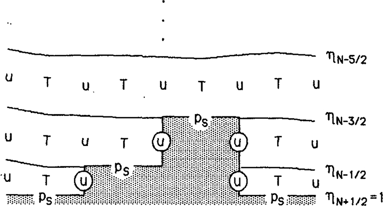
Figure 1
Example of a 2D representation of topography using the definitions in Equation 1 and 2. u represents x-component of velocity, T temperature, and N the number of model layers. From ( Janjić 1990).
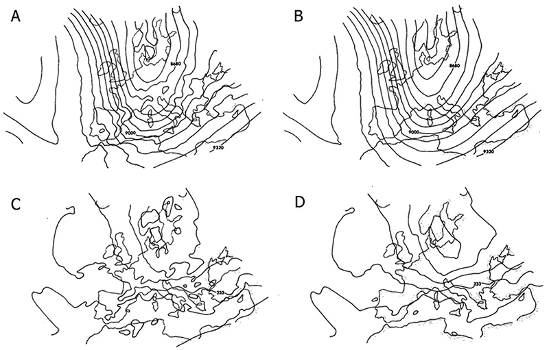
Figure 2
A 48-h simulation: A. 300 hPa geopotential heights using the sigma system; B. 300 hPa geopotential heights using the eta system; C. 300 hPa temperatures using the eta system; D. 300 hPa temperatures using the sigma system. Contour intervals are 80 m for geopotential heights, and 2.5°K for temperature. From ( Mesinger et al. 1988).
4 The Eta at NMC and NCEP
At the time of my 6 months visit to GFDL, it so happened there was an agreement between GFDL and the U.S. National Meteorological Center (NMC) for cooperation, that included a visit of a GFDL person to NMC. With no one, as I was told, of the possible GFDL candidates willing to spend time in a questionable Washington DC area neighborhood where NMC was located, I was asked if I would accept that mission. It looked excellent to me, what better place to promote the features of the model I had than the place where official U.S. forecasts were made?
A warm welcome was extended to me at NMC, with its then Director Bill Bonner, whom I knew from my UCLA time, personally instructing me how best to drive from my short-term rented apartment in northern Washington DC to the NMC's Camp Springs area southeast of the city. At NMC at the time a lot was expected from the so-called Nested Grid Model (NGM), created by the venerable Norman Phillips, who in 1974 left his MIT professorship and joined NMC as the “principal scientist” of the NMC Development Division.
One occasion I vividly recall form my early NMC time when chatting with Norm, as everyone would refer to Norman Phillips, at the entrance to his cubical, I asked him what Arakawa grid was he using in the NGM. “Here is our booklet”, he responded, handing me his and Jim Hoke's technical note on the NGM, “and you can find out”. I was astonished to realize that he did not know! Looking into the booklet I learned that he was using the D grid, the worst choice according to Arakawa.
As acknowledged in ( Mesinger et al. 1988), NMC people helped me install the code I brought on tape-as done at the time-from GFDL, and run additional experiments aimed at simulating the impacts of topography. Results were obviously sufficiently impressive to have the then National Weather Service (NWS) Director Ron McPherson, and others, see to it that the code is maintained, tested more ( Black 1988), and further developed, see Tom Black's words in Acknowledgements of ( Mesinger 2004). A crucial step in this further development was Zaviša Janjić's visit to NMC in 1987, during which he upgraded the then “minimum physics” package of the model, primarily by adding the Mellor-Yamada level 2.5 turbulence, level 2 in the lowest layer, and Betts-Miller convection scheme, with various modifications ( Janjić 1990).
Eventually the model code began to be referred to as the Eta model, note Tom Black's words just referred to. In addition to the NGM, there was at NMC the older limited area fine-mesh (LFM) model, with both models run operationally and results compared (e.g., Junker, Hoke & Grumm 1989). At somewhat later time Henry Juang brought to NMC his Regional Spectral Model (RSM) and obtained support to have it run on a regular basis.
Janjić's 1987 visit to NMC was followed by mine, of a year and a half, with the emphasis divided between additional model developments, mostly of its physics package, and verification efforts, all of these with continued assistance of Tom Black. Upgrades included a viscous sublayer over water added to the then surface layer scheme, so-called piecewise linear vertical advection of moisture, and in cooperation with Alan Betts, refinements of the Betts-Miller convection scheme. Verification efforts culminated in a three-way comparison of precipitation accuracy of the Eta vs. the NGM as run operationally, and vs. the NGM using the Eta's Betts-Miller convection scheme ( Mesinger et al. 1990). With the Eta demonstrating a clearly higher accuracy than the NGM across all intensity thresholds above the lightest ones, and the Eta convection scheme not having visibly helped the NGM become competitive to the Eta in the skill of intense precipitation, a strong implication was that it is the Eta dynamical core that is primarily responsible for its better skill.
Another Janjić's visit followed, with further development of the convection scheme, subsequently referred to as the Betts-Miller-Janjic (BMJ) scheme, a redesigned viscous sublayer scheme, different above land and water, and minor Mellor-Yamada (MY) changes (Janjić 1994). It should be noted however that the ( Janjić 1994) paper covers essentially only the material prior to the end of his just referred to visit, sometime in 1990, with only brief mentions of the developments after 1990.
When in early 1991 I rejoined what used to be the NMC's Development Division, reorganized so that it became the National Centers for Environmental Prediction/ Environmental Modeling Center (NCEP/EMC), its Director Eugenia Kalnay told me about a problem of the then semi-operational Eta. During the past winter it exhibited a “somewhat mixed performance over warm water”, occasional overdeepening of lows and widespread rain that did not verify. On a sensitive case of a real development experiments were subsequently performed, replacing the MY-2 (Mellor-Yamada level 2) of the lowest Eta layer by a standard Monin-Obukhov formulation, vs. what was referred to as “the l bulk” scheme, that I invented to replace the Janjić finite-difference type specification of the model's MY-2 lowest layer length scale scheme. The latter performed clearly better and very much removed the Eta problems referred to ( Mesinger (2010); Mesinger & Lobocki (1991)).
Another problem was identified by chance (serendipity?). A person running the Eta outside NCEP, Adrian Marroquin, complained about having no turbulence kinetic energy (TKE) above the planetary boundary layer (PBL). I had a look and noticed reasonable values in the forecast I looked at. The difference had to be in the code: Marroquin was using an older version which did not have the MY master length scale values I specified throughout the model atmosphere and thus also above the PBL, advised by Mark Helfand to do so, and addressing also other problems ( Mesinger 1993a). But having a look at the right place, I noticed a major oversight on the part of apparently all previous users of the MY-2.5, that made it next to impossible for TKE to be generated above the PBL ( Mesinger 1993b).
Following all these upgrades eventually the Eta became officially the U.S. operational regional model on 8 June 1993.
The NGM has been “frozen” prior to that already in 1991, but continued to be run, thus, inter alia, serving as a benchmark that could be used to assess the progress made. RSM also continued to be run beyond 1993, remaining a contender, note the statement of all the Development Division managers of that same year “A comparison with Regional Spectral Model (RSM) will determine possible replacement [of the Eta] by the RSM” ( Kalnay et al. 1993). It continued to be run until late 1997, with resolution about the same as that of the Eta, when in almost a 2-year comparison of more than a thousand forecasts the Eta demonstrated higher precipitation accuracy across all intensity thresholds, despite the RSM being run later with a 12-h more recent lateral boundary conditions ( Mesinger 2004, Figure 2).
As to the operational Eta, following a variety of enhancements and refinements made, in 1998 it achieved precipitation accuracy scores of its 24-48 h forecasts across all intensity thresholds higher than the NGM's scores of the 00-24 h forecasts.
The Eta accuracy over its U.S. domain was higher than that of the U.S. global model as well, and in 1997 a proposal was made for a “regional reanalysis” project, by the advisory committee of an existing global reanalysis project. The idea of such reanalyses, at the time one already having been performed, is to use a fixed model system and process all the data available starting with the beginning of satellite measurements, to obtain analyses of climate change not affected by the model and analysis changes. This, proposal to perform regional reanalysis using the Eta has eventually been accepted, funded, and done for its initial 25-yr retrospective period, and continues to be performed in near-real time as we speak. Paper describing the method and results of these first 25 years of data, ( Mesinger et al. 2006), is frequently cited, so that in Google Scholar as this is being written it has more than 3800 citations.
However, a problem with the Eta has been noticed that had a rather negative impact on its reputation. ( Gallus & Klemp 2000) reported on the problem of a nonhydrostatic eta code in simulating flow over a 2D bell-shaped topography, of flow separation off the top of the topography instead of a descent down the lee slope. In addition, an experimental 10-km Eta forecast failed to forecast an intense downslope windstorm in the lee of the Wasatch Mountain, while a sigma system MM5 model did well ( McDonald et al. 1998). With these and other considerations, when replacing the referred to 10-km Eta by an 8-km Nonhydrostatic Mesoscale Model (NMM), using terrain-following coordinate, an announcement was made that “This choice [of the vertical coordinate] will avoid the problems ... with strong downslope winds and will improve placement of precipitation in mountainous terrain” (DiMego, personal communication, 19 July 2002).
Accordingly, upgrades of the Eta were discontinued, and in addition a more advanced data assimilation system has been developed for the NMM. Eventually in 2006 a so-called “parallel” was run, of four+ months of forecasts of the operational Eta system, and the newly developed NMM system, at the same domains and resolution. The Eta performed clearly better with precipitation skill scores, the more so the longer-range forecasts were looked at (e.g., Mesinger & Veljovic 2017). There was little else in terms of objective scores that would be favoring the NMM ( DiMego 2006). Over higher topography western contiguous United States, the Eta remained more accurate in both 2-m temperatures and 10-m winds, despite its poorer vertical resolution there resulting from the change in the vertical coordinate ( Mesinger 2022). Nevertheless, perhaps understandably, decision was made to have the NMM be the next U.S. operational regional model.
5 The Eta Outside NCEP
With the Eta demonstrating accuracy as summarized no wonder it was used in various ways in some countries outside the United States. In 1994-1998 it was the primary experimental tool of international summer schools organized in Krivaja, Bačka Topola, by the Federal Hydrometeorological Institute, Belgrade, sponsored and partly supported by WMO. It was used in three two-week workshops/ conferences on regional modeling organized by the International Centre for Theoretical Physics (ICTP) near Trieste, Italy, 2002, 2005, and 2008.
The most extensive use of the Eta outside NCEP was at Center for Weather Prediction and Climate Studies (CPTEC), an agency of National Institute for Space Research (INPE), Cachoeira Paulista, SP, Brazil, as this is being written only INPE. Two CPTEC people visited NMC in 1996 and have taken the Eta code to Brazil. One of them was Sin Chan Chou who continued using it and organized a dedicated group using the Eta for short range forecasts and as a regional climate model (RCM). As this is written Chou just recently, past September, organized for the 7th time an Eta model workshop with participants being taught to run the model and make experiments. Twice it was the model of choice of an U.N. economic commission, CEPAL, covering Latin America and the Caribbean, for training workshops on climate change, hosted by CPTEC.
CPTEC, following NCEP's 2006 decision of replacing the Eta, has become kind of a “primary home” of the Eta, not only for hosting events but also in taking part in contributions to the further development of the model. Thus, the paper summarizing the design of the model as of 2011, ( Mesinger et al. 2012), of 11 coauthors includes five who are or were resident of Brazil.
This presentation will continue with illustrations of some of the major advancements following 2006. To address the “Gallus-Klemp problem” of the Eta, I had a long-standing idea on my “to do list” what needs to be done. Since Gallus and Klemp ascribed the problem to the existence of step corners of the step topography Eta, I was going to change the discretization so that the velocity cells just above the corners have sloping bottoms, as illustrated in the schematic of Figure 3.
Once a version of the code using “sloping steps” was put together a test was done using an 8-km/60-layer code over a domain of the western United States and running a 48-h forecast. Obtained temperatures of the lowest layer T cells are shown in Figure 4. Two or three spots all in mountain basins are seen responsible for the choice of the NCAR graphics routine of the plotting interval of 10°K, one of them in southwestern Montana, with the temperatures below 180°K. Another in western Alberta, not much warmer than that.
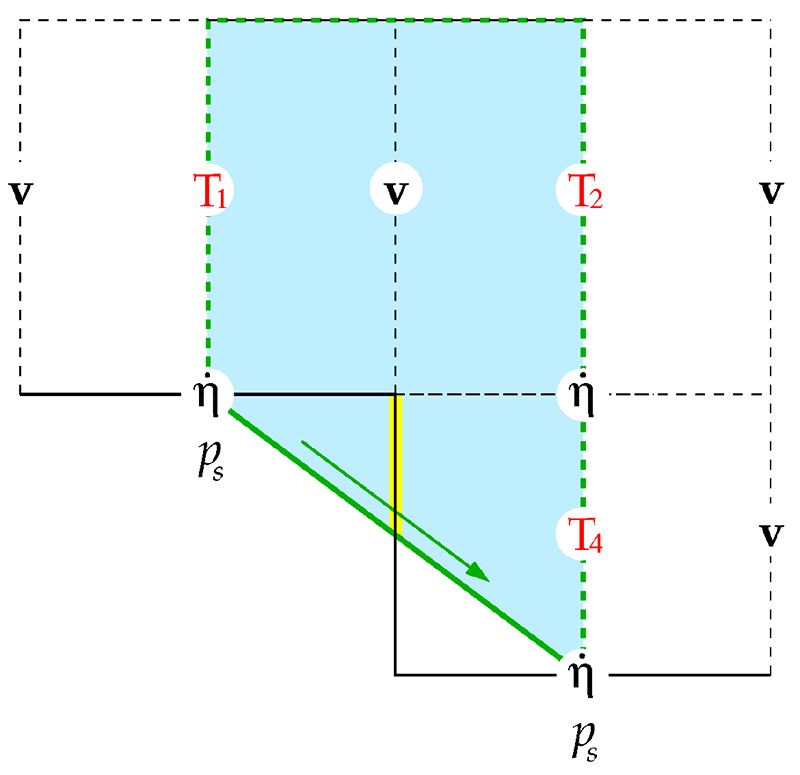
Figure 3
Schematic illustrating the “sloping steps” Eta discretization. The vertical topography side below the velocity ( v) cell in the middle is replaced by a sloping side going from the left to the right surface pressure (p S) points. Symbols T denote temperature cells, η denotes the eta coordinate, with dot (˙) above a symbol standing for the time derivative. From ( Mesinger et al. 2012).
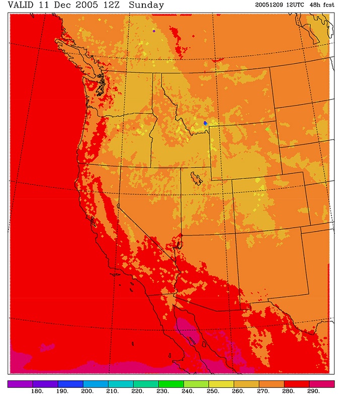
Figure 4
Temperatures (K) of the lowest temperature cells of a 48-h forecast with the “sloping steps” Eta, using a finite-difference “Lorenz-Arakawa” centered slantwise temperature advection scheme.
Given that such temperatures do not occur in the real world, understanding what happened was obviously needed. It was not hard to get the idea that the finite-difference vertical advection scheme, used for slantwise temperature advection such as between cells T 1 and T 4 in Figure 3, is a good candidate to be responsible.
The centered finite-difference scheme used for the slantwise advection in calculating temperatures of Figure 4 was the Equation 3:
d/dt being the time derivative, the eta vertical velocities, 𝜂 , being defined at cell interfaces, the overbar standing for two-point averaging in the direction indicated, and ∆ denoting the finite difference in the direction of the η.
Suppose the left half of the schematic of Figure 1 were the exit region of a basin with predominant flow to the right and somewhat upward. According to the Equation 3 the temperature change due to vertical advection is the average of contributions from the top and the bottom sides of T cells. If a temperature inversion were to develop between the two leftmost and lower T cells, then the vertical advection contribution from their interface would cool both cells, but for the lower of them would be the only contribution, thus tending to increase the inversion, amplifying its cooling, feeding on itself. An instability like mechanism would be established, for a physically wrong reason.
It was easy to avoid the problem. As we know the velocity across the upper half of what was a vertical step, yellow in the schematic of Figure 3, we also know the mass of air moving in the time step from cell T 1 to T 4, so that it is straightforward to calculate the temperature changes due to the slantwise advection in a Lagrangian way. This was coded instead of the use of Equation 3, and a realistic temperature forecast was obtained instead of that of Figure 4.
However, the scheme Equation 3 was used not only for slantwise advection, but for the vertical advection of the main prognostic variables, v and T, as well. Being now aware of the scheme's problem at the lowest cells, I have changed the vertical advection of v and T to the finite-volume scheme that the model was already using for moisture ( Mesinger & Jovic 2002). It is a scheme that respecting the finite-volume meaning of prognostic values as cell averages, adjusts slopes of cells toward values at neighboring cells, but without creating new minima or maxima and keeping them linear inside cells. Thus, the term “piecewise linear” is used. Advection can then be performed using velocities at cell boundaries.
An unexpected reward came from that change, in addressing the model's difficulty with downslope windstorms. When the change was made experiments were in progress with cases of intense downslope windstorms in the lee of the Andes. Two sections of synoptic maps illustrating one of these cases are shown in Figure 5. The case is the same as in Section 9 of ( Mesinger et al. 2012). Warming of 24°C is seen at the station San Juan, about the middle of the maps, from 1200 to 1800 UTC. Warmings of that type are known in the Alpine region under the name “foehn”, in the lee of the Andes their name is “zonda” (e.g., Antico, Chou & Brunini 2021, and references therein).
The “reward” just referred to is illustrated by the two plots of Figure 6. The one on the left shows the result of the forecast using Equation 3 for the slantwise as well as the vertical advection, while the one on the right shows the result with Equation 3 replaced by the slantwise Lagrangian and the finite-volume piecewise linear vertical advections. Warming in the zonda region is thereby seen increased by more than 4°K and occurs in one might say “the right place”. But to get back to the total warming, compared to the 24 h forecast (not shown) the warming of Figure 6 at San Juan is comfortably more than 20°K. Thus, notwithstanding the difference of 33 vs. 30 h, this zonda effort can be declared a success.
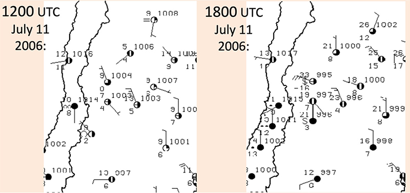
Figure 5
Sections of surface maps illustrating a case of an intense “zonda” windstorm in the lee of the Andes. Warming from 9 to 33°C in 6 h is seen at the station San Juan, 630 m above sea level, close to the middle of the above sections. Valid times are displayed in the top left corner of the maps.
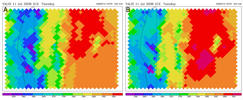
Figure 6
Forecast lowest cell temperatures (K) at 33 h of the case discussed in Section 9 of ( Mesinger et al. 2012) : A. Result obtained using Equation 3 for both the slantwise and the vertical advection; B. Result with these advections replaced by the finite-volume versions . The roughly vertical line on the left sides of the plots is the Chile-Argentina border, while the straight line is the 70°W meridian. The small cross to the right of the centers of plots shows the place of the San Juan station.
Nevertheless, it is the flow separation issue pointed out by ( Gallus & Klemp 2000) that was quoted the most as the weakness warning people to stay away from the eta system, e.g., five citations listed in ( Mesinger 2004). Thus, it required attention, and it was on 9 March 2002 that I worked out a plan how to address it. I could look up this date because I recall I was then travelling on a ship from a meeting on Awaji Island to Osaka. My plan involved defining slopes at the bottoms of v cells, using the topography values of four surrounding z S points. Thereby the step corners of the eta topography according to ( Gallus & Klemp 2000) responsible for the flow separation would be eliminated, and presumably the Gallus-Klemp Eta problem as well.
Implementing all the steps of this plan was not straightforward, with work done at several places. It began during my visits to the Abdus Salam International Centre for Theoretical Physics (ICTP), continued at NCEP/EMC, and was mostly completed at CPTEC. Assistance was needed in handling the code I wrote, or in generating plots as those of Figure 6, and was at ICTP and EMC obtained from Dušan Jović, and at CPTEC from the Sin Chan Chou's group, primarily Jorge Gomes. A major code bug I made was eventually discovered by Ivan Ristić of the “Weather2” Belgrade company, and the code then seemed to work fine. But the flow separation in the Gallus-Klemp experiment of 2D bell-shaped topography ( Mesinger et al. 2012, Figure 3), while visibly improved, was not completely removed.
An unusual help came in 2013 from Sandra Morelli, of the University of Modena, Italy. Morelli informed me of noticing “something strange” in the code of the so-called horizontal diffusion, code modelers use either to avoid unwanted noisiness of fields, or to simulate impact of unresolved motions, the latter in the case of the Eta. This in agreement with ( Mellor 1985), pointing out that horizontal diffusion should not be looked at as a turbulence closure mechanism but instead needs to be viewed as a substitute mechanism for unresolved horizontal advective processes.
“Something strange” was leftover code from a previous sigma version that was with the eta coordinate not active, but a look at the right place was enough to see the problem. Horizontal diffusion code was not made aware of the “sloping steps” and was responsible for some remaining flow separation. This being addressed, flow over a 2D bell-shaped topography was obtained as in the right-hand plot of Figure 7. The left-hand plot is (c) of Figure 6 of ( Gallus & Klemp 2000), which they obtained using an artificial modification of the code to remove the impact of the step corners they found responsible for the flow separation problem.
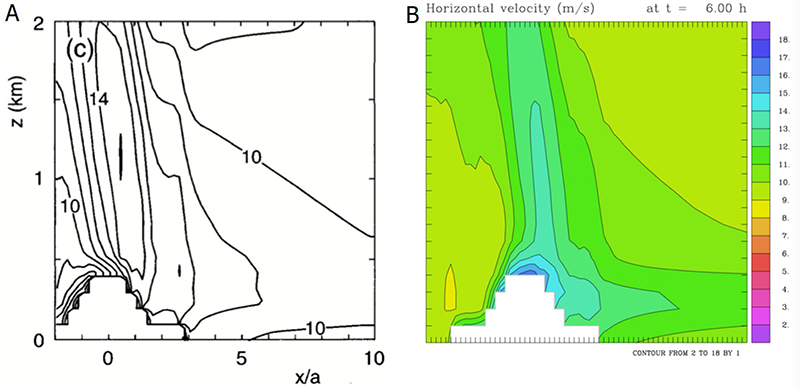
Figure 7
Simulation of the Gallus-Klemp experiment with the Eta code. A. Plot (c) of Figure 6 of (Gallus & Klemp 2000); B. Result obtained using the cut cell Eta code allowing for velocities at slopes in the horizontal diffusion scheme. From ( Mesinger & Veljovic 2017).
The routine used for our right-hand plot of Figure 7 did not allow for slopes, so they are not visible in the topography of Figure 7. Compared to the linear solution one could be concerned with the maximum on top of the mountain, but I am confident this could be improved with slopes over more than one cell if this were felt to be an issue of sufficient priority.
6 Eta as RCM and its Large-Scale Skill
While the Eta has been set up and tested as a global model on a cubed-sphere and on an octagonal grid ( Zhang & Rančić 2007; Latinović et al. 2019), its use almost exclusively was as a limited area model (LAM), covered in two preceding sections. As stated earlier, as RCM it enjoyed extensive use for a variety of purposes mostly over South American domains (e.g., Chou et al. 2012, 2014a, 2014b; Lyra et al. 2018; Chou et al. 2020, all with references to many others).
One point can be stressed here. It is almost universally believed that the nested model should improve on smaller scales, while it should accept “large scales” as they are in its driver global model. Consequently, so called Davies’ relaxation lateral boundary conditions are applied, forcing variables in some rows around the boundary to conform to the driver model values, completely at the boundary, and less and less toward the inside of the domain. Very often investigators also apply the so-called large scale or spectral nudging inside the domain, forcing the integration variables not to depart much from those of the driver model.
It is hard to see a scientific basis for these practices, but there is a scientific basis for having fewer conditions prescribed on the outflow than on the inflow parts of the boundary (e.g., Mesinger & Veljovic 2013). From its very beginning, following one option suggested by ( Sundström 1973), this is done in the Eta ( Mesinger 1977). Hundreds of thousands of the Eta forecasts performed at NCEP, CPTEC, and other places, with no lateral boundary condition (LBC) problems encountered, testify to the relaxation LBCs being unnecessary. For reasons just mentioned, they should in addition be expected to be harmful.
As to the large-scale nudging, while the global driver model might be equipped with components and feedbacks missing in a LAM or RCM, if we consider just the atmospheric motion, impact of these missing components can be received via the inflow LBCs but large scales inside the LAM domain could still be improved if the LAM has some advantage over its driver model. The advantage could be higher resolution but can also be a dynamical core better in some ways, or both, but hardly better parameterizations because global models require considerable parameterization efforts.
As an example, in Figure 8 average wind speed at 250 hPa of an Eta 21-member ensemble is shown, top right, driven by a European Centre for Medium-Range Weather Forecasts (ECMWF, or EC) ensemble, with its average wind speed at the same height at bottom left, both at 4.5-day lead time. Space resolution of the Eta ensemble was about the same as that of its driver EC ensemble. EC analysis valid at the same time is shown at the bottom right, and the average wind speed at the same height of the Eta ensemble switched to use sigma, Eta/sigma, top left. Compared to the driver ensemble, note the more accurate Eta's northeastward extension of the New England jet streak of > 45 m/s, as well as the more accurate southeastward extension of the one over the Canadian Rockies, past all the three major Canadian lakes of the area. Interestingly, that last advantage is achieved by the Eta/sigma ensemble just as well, this not being to the same extent the case for the former.
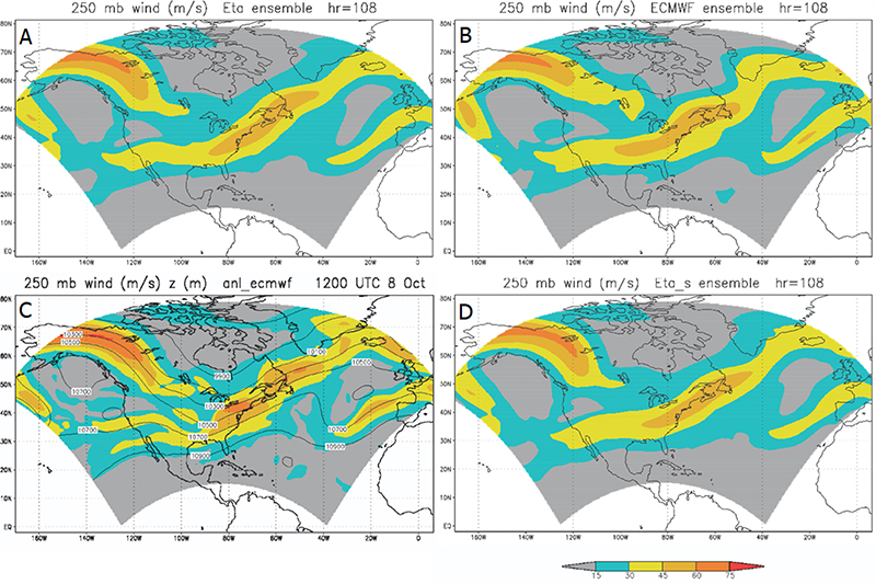
Figure 8
A. Averages of 4.5-day forecast 250 hPa wind speeds (m/s) of a 21 member Eta ensemble; B. Same, but of its EC driver ensemble members; C. The EC verification analysis; D. Same, but of the Eta ensemble switched to use sigma. Analysis includes geopotential height contours (m). From ( Mesinger & Veljovic 2020).
( Mesinger & Veljovic 2020) present more detail, including counts of wins in comparing three pairs of ensembles, Eta vs. EC, Eta/sigma vs. EC, and Eta vs. Eta/sigma, and using three verification measures. With each of them at 4.5 days all 21 Eta members had better skill scores of 250 hPa wind speeds than their driver EC members, repeatedly prior and about that time for two of them, bias adjusted Equitable Threat Score (ETSa, Mesinger 2008) and RMS difference. With the third score, “symmetric extreme dependency score” (SEDS), proposed by ( Hogan, O’Connor & Illingworth 2009), dominant results of the Eta following the initial two days were displayed as well, all the way out to about the 18-day time. The first about two days the Eta was at a disadvantage certainly because of its initial conditions’ interpolation off those of the EC driver members.
Identifying the reasons why the Eta switched to use the sigma coordinate, Eta/sigma, tends to achieve better scores than its EC drivers is a challenging issue. Of several candidates listed in ( Mesinger & Veljovic 2020), zonda results of Figure 6 suggest the finite-volume vertical advection to perhaps be the major one.
7 Concluding Comments
Weather and climate models require many components and are nowadays never developed by a single person. But if a model that in terms of its dynamical core features was developed primarily by only two people achieves results at least comparable with a model of a major international institution, one might wonder why this has happened. Regarding the model of the institution referred to, note the words of a recent review of numerical methods in atmosphere and ocean models: “Although spectral transform methods are being predicted to be phased out, the current spectral model at the European Centre for Medium-Range Weather Forecasts... is the benchmark to beat, and it is not clear that any of the new developments are ready to replace it” ( Côté et al. 2015).
In this text two features have been listed with results illustrated that contributed to the Eta skill but are absent in the EC model. One is the Eta vertical coordinate resulting in quasi-horizontal coordinate surfaces, eliminating thus a possibility for large pressure gradient force errors.
Another is the finite-volume slantwise and vertical advection. They not only avoided the false advection from below ground of the finite-difference scheme used previously and made a crucial contribution to the simulation of the zonda windstorm, but they also achieved consistency with the finite-volume property of the Eta Arakawa horizontal advection. This I believe has been essential for the successful performance of the Eta model as shown.
Acknowledgements
Many people in numerous ways enabled the today's existence and skill of the Eta model, its code, and its results. To list only some, Zaviša Janjić, Lazar Lazić, Tom Black, Eugenia Kalnay, Dušan Jović, Sin Chan Chou, Jorge Gomes, Sandra Morelli, Ivan Ristić, Katarina Veljović, too many more to mention individually, and to all of them goes my appreciation and heartfelt gratitude. Suggestions of the two reviewers, one being Sin Chan Chou, are much appreciated, for having helped include some useful information, and improving the readability of the text. This article was submitted at the suggestion of Claudine Dereczynski, who in numerous ways helped the existence and life of the “Eta community” and made contributions to its spirit that I am convinced many members including myself will never forget.
References
Antico, P.L., Chou, S.C. & Brunini, C.A. 2021, 'The foehn wind east of the Andes in a 20-year climate simulation', Meteorology and Atmospheric Physics, vol. 133, pp. 317-30, DOI:10.1007/s00703-020-00752-3.
Arakawa, A. 1966, 'Computational design for long-term numerical integration of equations of fluid motion: Two dimensional incompressible flow. Part I', Journal of Computational Physics, vol. 1, no. 1, pp. 119-43, DOI:10.1016/0021-9991(66)90015-5.
Arakawa, A. & Lamb, V.R. 1977, 'Computational design of the basic dynamical process of the UCLA general circulation model', in J. Chang (ed.), Methods in Computational Physics, Academic Press, 17, pp. 173-265.
Black, T.L. 1988, The step-mountain eta coordinate regional model: a documentation, NOAA/NWS National Meteorological Center, < http://ftp1.cptec.inpe.br/pesquisa/grpeta/petamdl/Publications/Black.1988+_EtaDocumentation.pdf>
Chang, J. (ed.). 1977, General Circulation Models of the Atmosphere: Methods in Computational Physics, Academic Press.
Charney, J.G., Fjørtoft, R. & von Neumann, J. 1950, 'Numerical integration of the barotropic vorticity equation', Tellus, vol. 2, no. 2, pp. 237-54, DOI:10.1111/j.2153-3490.1950.tb00336.x.
Chou, S.C, Dereczynski, C., Gomes, J.L., Pesquero, J.F., de Avila, A.M.H., Resende, N.C., Alves, L.F., Ruiz-Cárdenas, R., de Souza, C.R. & Bustamante, J.F.F. 2020, 'Ten-year seasonal climate reforecasts over South America using the Eta regional climate model', Anais da Academia Brasileira de Ciências, vol. 92, no. 3, pp. 1-24, DOI:10.1590/0001-3765202020181242.
Chou, S.C., Lyra, A, Mourão, C, Dereczynski, C, Pilotto, I., Gomes, J., Bustamante, J., Tavares. P., Silva, A., Rodrigues, D., Campos, D., Chagas, D., Sueiro, G., Siqueira. G., Nobre, P. & Marengo, J. 2014a, 'Evaluation of the Eta simulations nested in three global climate models', American Journal of Climate Change, vol. 3, no. 5, pp. 438-454, DOI:10.4236/ajcc.2014.35039.
Chou, S.C., Lyra, A., Mourão, C., Dereczynski, C., Pilotto, I., Gomes, J., Bustamante, J., Tavares, P., Silva, A., Rodrigues, D., Campos, D., Chagas, D., Sueiro, G., Siqueira, G. & Marengo, J. 2014b, 'Assessment of climate change over South America under RCP 4.5 and 8.5 downscaling scenarios', American Journal of Climate Change, vol. 3, no. 5, pp. 512-27, DOI:10.4236/ajcc.2014.35043.
Chou, S.C., Marengo, J.A., Lyra, A., Sueiro, G., Pesquero, J., Alves, L.M., Kay, G., Betts, R., Chagas, D., Gomes, J.L., Bustamante, J. & Tavares, P. 2012, 'Downscaling of South America present climate driven by 4-member HadCM3 runs', Climate Dynamics, vol. 38, no. 3-4, pp. 635-53, DOI:10.1007/s00382-011-1002-8.
Côté, J., Jablonowski, C., Bauer, P. & Wedi, N. 2015, 'Numerical methods of the atmosphere and ocean', in Seamless Prediction of the Earth System: From Minutes to Months, World Meteorological Organization WMO No. 1156 pp. 101-24.
DiMego, G. 2006, WRF-NMM & GSI Analysis to replace Eta Model & 3DVar in NAM Decision Brief, U.S. National Centers for Environmental Prediction < https://www.emc.ncep.noaa.gov/WRFinNAM/ Update_WRF-NMM_replacing_Eta_in_NAM2.pdf>.
Egger, J. 1972, 'Numerical experiments on the cyclogenesis in the Gulf of Genoa', Beiträge zur Physik der Atmosphäre, vol. 45, pp. 20-346.
Gallus Jr., W.A. & Klemp, J.B. 2000, 'Behavior of flow over step orography', Monthly Weather Review, vol. 128, no. 4, pp. 1153-64, DOI:10.1175/1520-0493(2000)128%3C1153:BOFOSO%3E2.0.CO;2.
Hogan, R.J., O’Connor, E.J. & Illingworth, A.J. 2009, 'Verification of cloud-fraction forecasts', Quarterly Journal of the Royal Meteorological Society, vol. 135, no. 643, pp. 1494-511, DOI:10.1002/qj.481.
Janjić, Z.I. 1984, 'Nonlinear advection schemes and energy cascade on semi-staggered grids', Monthly Weather Review, vol. 112, no. 6, pp. 1234-45, DOI:10.1175/1520-0493(1984)112%3C1234:NASAEC%3E2.0.CO;2.
Janjić, Z.I. 1990, 'The step-mountain coordinate: physical package', Monthly Weather Review, vol. 118, no. 7, pp. 1429-43, DOI:10.1175/1520-0493(1990)118%3C1429:TSMCPP%3E2.0.CO;2.
Janjić, Z.I. 1994, 'The step-mountain eta coordinate model: Further developments of the convection, viscous sublayer, and turbulence closure schemes', Monthly Weather Review, vol. 122, no. 5, pp. 927-45, DOI:10.1175/1520-0493(1994)122%3C0927:TSMECM%3E2.0.CO;2.
Junker, N.W., Hoke, J.E. & Grumm, R.H. 1989, 'Performance of NMC's regional models', Weather and Forecasting, vol. 4, no. 3, pp. 368-90, DOI:10.1175/1520-0434(1989)004%3C0368:PONRM%3E2.0.CO;2.
Kalnay, E., Baker, W., Kanamitsu, M., Petersen, R., Rao, D.B. & Leetmaa, A. 1993, 'Modeling plans at NMC for 1993-1997', 13th Conference on Weather Analysis and Forecasting, Vienna, VA, American Meteorological Society, pp. 340-43.
Kreiss, H. & Oliger, J. 1973, Methods for the Approximate Solution of Time-Dependent Problems, WMO/ICSU Joint Organizing Committee.
Latinović, D., Chou, S.C., Rančić, M., Medeiros, G.S. & Lyra, A.A. 2019, 'Seasonal climate and the onset of the rainy season in western-central Brazil simulated by Global Eta Framework model', International Journal of Climatology, vol. 39, no. 3, pp. 1429-45, DOI:10.1002/joc.5892.
Lyra, A., Tavares, P., Chou, S.C., Sueiro, G., Dereczynski, C.P., Sondermann, M., Silva, A., Marengo, J. & Giarolla, A. 2018, 'Climate change projections over three metropolitan regions in Southeast Brazil using the non-hydrostatic Eta regional climate model at 5-km resolution', Theoretical and Applied Climatology, vol. 132, pp. 663-82, DOI:10.1007/s00704-017-2067-z.
McDonald, B.E., Horel, J.D., Stiff, C.J. & Steenburgh, W.J. 1998, 'Observations and simulations of three downslope wind events over the northern Wasatch Mountains', 16th Conference on Weather Analysis and Forecasting, American Meteorological Society, Phoenix pp. 62-4.
Mellor, G.L. 1985, 'Ensemble average, turbulence closure', in S. Manabe (ed.), Advances in Geo- physics, Issues in Atmospheric and Ocean Modeling. Part B: Weather Dynamics, Academic Press, pp. 345-57.
Mesinger, F. 1977, 'Forward-backward scheme, and its use in a limited area model', Contributions to Atmospheric Physics, vol. 50, pp. 200-10.
Mesinger, F. 1984, 'A blocking technique for representation of mountains in atmospheric models', Rivista di Meteorologia Aeronautica, vol. 44, pp. 195-202.
Mesinger, F. 1993a, Sensitivity of the definition of a cold front to the parameterization of turbulent fluxes in the NMC's Eta Model, Research Activities in Atmospheric and Oceanic Modelling, WMO, Geneva, pp. 436-8.
Mesinger, F. 1993b, Forecasting upper tropospheric turbulence within the framework of the Mellor-Yamada 2.5 closure, Research Activities in Atmospheric and Oceanic Modelling, WMO, Geneva, CAS/JSC WGNE Rep. 18, pp. 428-9.
Mesinger, F. 2004, 'The Eta model: design, history, performance, what lessons have we learned?', Symposium on the 50th anniversary of operational numerical weather prediction, University of Maryland, 14-17 June 2004, < https://www.ncep.noaa.gov/nwp50/Agenda/Tuesday/>
Mesinger, F. 2008, 'Bias adjusted precipitation threat scores', Advances in Geosciences, vol. 16, pp. 137-42, DOI:10.5194/adgeo-16-137-2008.
Mesinger, F. 2010, 'Several PBL parameterization lessons arrived at running an NWP model', International Conference on Planetary Boundary Layer and Climate Change, vol. 13, e012005, DOI: 10.1088/1755-1315/13/1/012005.
Mesinger, F. 2022, Vertical resolution of the surface layer versus finite-volume and topography issues, Boundary-Layer Meteorology, vol. 187, no. 5, DOI:10.1007/s10546-022-00745-2.
Mesinger, F. & Arakawa, A. 1976, Numerical methods used in atmospheric models , WMO/ICSU Joint Organizing Committee, Geneva, Switzerland. GARP Publications Series no. 17, vol. 1.
Mesinger, F., Black, T.L., Plummer, D.W. & Ward, J.H. 1990, 'Eta model precipitation forecasts for a period including tropical storm Allison', Weather and Forecasting, vol. 5, no. 3, pp. 483-93, DOI:10.1175/1520-0434(1990)005%3C0483:EMPFFA%3E2.0.CO;2.
Mesinger, F., DiMego, G., Kalnay, E., Mitchell, K., Shafran, P.C., Ebisuzaki, W., Jovic, D., Woollen, J., Rogers, E., Berbery, E.H., Ek, M.B., Fan, Y., Grumbine, R., Higgins, W., Li, H., Lin, Y., Manikin, G., Parrish, D. & Shi, W. 2006, 'North American Regional Reanalysis', Bulletin of the American Meteorological Society, vol. 87, no. 3, pp. 343-60, DOI:10.1175/BAMS-87-3-343.
Mesinger, F., Chou, S.C., Gomes, J., Jovic, D., Bastos, P., Bustamante, J.F., Lazic, L., Lyra, A.A., Morelli, S., Ristic, I. & Veljovic, K. 2012, 'An upgraded version of the Eta model', Meteorology and Atmospheric Physics, vol. 116, no. 3-4, pp. 63-79, DOI:10.1007/s00703-012-0182-z.
Mesinger, F., Janjic, Z.I., Nickovic, S., Gavrilov, D. & Deaven, D.G. 1988, 'The step-mountain coordinate: model description, and performance for cases of Alpine lee cyclogenesis and for a case of an Appalachian redevelopment', Monthly Weather Review, vol. 116, no. 7, pp. 1493-518, DOI:10.1175/1520-0493(1988)116%3C1493:TSMCMD%3E2.0.CO;2.
Mesinger, F. & Jovic, D. 2002, The Eta slope adjustment: Contender for an optimal steepening in a piecewise-linear advection scheme? Comparison tests, NOAA/NCEP Office Note 439, US Department of Commerce, Washington.
Mesinger, F. & Lobocki, L. 1991, 'Sensitivity to the parameterization of surface fluxes in NMC’s eta model', 9th Conf on Numerical Weather Prediction, American Meteorological Society, Denver, pp. 213-6.
Mesinger, F. & Veljovic, K. 2013, 'Limited area NWP and regional climate modeling: a test of the relaxation vs Eta lateral boundary conditions', Meteorology and Atmospheric Physics, vol. 119, no. 1-2, pp. 1-16, DOI:10.1007/s00703-012-0217-5.
Mesinger, F. & Veljovic, K. 2017, 'Eta vs. sigma: Review of past results, Gallus-Klemp test, and large-scale wind skill in ensemble experiments', Meteorology and Atmospheric Physics, vol. 129, no. 6, pp. 573-93, DOI:10.1007/s00703-016-0496-3.
Mesinger, F. & Veljovic, K. 2020, 'Topography in weather and climate models: Lessons from cut-cell Eta vs. European Centre for Medium-Range Weather Forecasts experiments', Journal of the Meteorological Society of Japan, vol. 98, no. 5, pp. 881-900, DOI:10.2151/jmsj.2020-050.
Phillips, N.A. 1959, 'An example of non-linear computational instability', in The Atmosphere and the Sea in Motion, Rockefeller Institute Press, New York, pp. 501-4.
Richtmyer, R.D. & Morton, K.W. 1967, Difference Methods for Initial-Value Problems, Interscience Publishers, New York.
Salmon, R. 2004, 'Poisson-Bracket approach to the construction of energy- and potential-enstrophy-conserving algorithms for the shallow-water equations', Journal of the Atmospheric Sciences, vol. 61, no. 16, pp. 2016-36, DOI:10.1175/1520-0469(2004)061%3C2016:PATTCO%3E2.0.CO;2.
Sundström, A. 1973, Theoretical and practical problems in formulating boundary conditions for a limited area model, Stockholm University, Stockholm.
Zhang, H. & Rančić, M. 2007, 'A global Eta model on quasi-uniform grids', Quarterly Journal of the Royal Meteorological Society, vol. 133, no. 623, pp. 517-28, DOI:10.1002/qj.17.
Data availability statement
Funding information
Author notes
E-mail: fedor.mesinger@gmail.com
Conflict of interest declaration