1. Introduction

According to the World Bank (undated), Mexico is classified as an upper middle income country. Regarding the Gini index, it fell from 0.460 in 2018 to 0.435 in 2022. However, social disparities prevail. In 2022, 46.8 million people were living in poverty, equivalent to 36.3% of the population. Within this group, inhabitants under extreme poverty rose from 8.7 to 9.1 million during the same time period (Coneval, 2023).

Two factors pertain to the above mentioned backwardness. On the one hand, overcrowded dwellings prevail. Absence of basic services is an additional factor. In 2022, 9.1% of the population faced the shortcomings specified in the first constraint, while 17.8% did not have access to basic services, according to the last source. These disadvantages underline the need of residential building construction for improving living standards.

According to the North American Industry Classification System (NAICS, 2022), residential building construction comprises: i) new single-family housing construction; ii) new multifamily housing construction; iii) new housing for-sale builders and iv) residential remodelers. In its turn, nonresidential building construction is integrated by commercial and institutional building constructions. ¹ However, Inegi (undated) does not break down data beyond residential and non-residential building construction.

In what follows, every reference of residential or nonresidential building construction will be referred, for short, as residential or nonresidential construction. In both cases, they allude to buildings. Other types of nonresidential constructions which do not pertain to buildings, for instance, heavy and civil engineering are being excluded in the present analysis.

Macroeconomic accounts are available for both sectors of this construction industry, providing a set of economic elements making possible an examination of its behavior. Based on this information, a model is presented in the second part of this paper. The following analysis is made considering both residential and nonresidential construction activities. Initially, gross output growth of this industry as well as regarding the rest of the Mexican economy is being estimated.

Afterwards, employment is measured by job posts, following the unit of account provided by the statistical agency. Intermediate consumption is analyzed on its own, while its effect in employment is measured. Compensation of employees is singled out to estimate its trend. The wage rate is made dependent on the gross operational surplus; this last one as a share of gross value added. The wedge between product wages and real wages is gauged, due to inflation disparities. In the last section, conclusions are put forward.

2. A model

The following set of equations evaluate residential and nonresidential construction. Initially, gross output growth is estimated in these two sectors. In addition, it is calculated for the rest of the economy by means of the following equation:

where ls means least squares, go stands for gross output, and p_goi is the gross value added deflator. In addition, i = 1, 2, 3, while 1 stands for residential construction, 2 for nonresidential construction, and 3 for the remaining sectors of the economy. The variable c is the intercept, indicating the growth rate. The symbol ∆ indicates that the dependent variable whose growth is being estimated is stationary, while log stands for logarithm and ls stands for least squares.

The growth of job posts, as a proxy of employment, is estimated:

where jp represents job posts and i = 1, 2, as 1 is referred to residential construction, while 2 is for nonresidential construction. The intercept is specified with the letter c, to indicate the rate of growth. The symbol ∆ indicates that the variable under estimation is within the unit circle.

The expansion of physical circulating means of production is to be calculated as follows:

where ic refers to intermediate consumption and p_ici is the deflator for this variable. Values of 1 and 2 are taken by subindex 𝒾. Number 1 and 2 stand for residential and nonresidential construction, respectively. The letter c stands for the intercept, indicating the growth rate. The variable under estimation is to be stationary, as indicated by the ∆ symbol.

The pace of intermediate consumption expansion vis-à-vis the number of job posts is to be estimated. If economies of scale are growing, a coefficient below one is expected, and vice versa. The proposed equation is:

as jp represents the job posts and ic is the value of intermediate consumption. The subinde x i = 1, 2. Number 1 is to represent residential construction, while 2 refers to nonresidential construction. The letter c is the intercept.

The estimated level of wages is to be related with the gross operational surplus as a share of gross value added.

An average wage is estimated by dividing the compensation of labor (cl_i) by the number of job posts (jp_i), adjusted for inflation by the gross value added deflator (p_{gva i}). Subindex 𝒾 takes the values 1 and 2. Therefore, the first expression is a proxy for average wages, duly deflated. In turn, gos refers to gross operational surplus, while gva represents gross value added. Number 1 is referred to residential construction and number 2 corresponds to nonresidential construction. This expression estimates the effect of gross operational surplus as a share of gross value added, in the level of average wages. A negative coefficient is expected, as a higher share of gross operational surplus of the gross value added, would take place at the expense of the above mentioned wages.

The gross value added inflation, as well as the consumer price index are presented as a ratio whose growth is being estimated.² Therefore, a wedge which could arise between both, is to be estimated as follows:

where p_{gva i} is the price index for gross value added, while p_cpi is the consumer price index. The subindex takes the values of 1 and 2, referring to residential and nonresidential construction, respectively. If the coefficient is above one, inflation regarding the value of labor power in construction would be higher than the purchasing power of the laborer demanding final goods, and vice versa.

3. Data

The data for the above model is made available by the local statistical office, i.e., Instituto Nacional de Estadística y Geografía (Inegi, undated). The variables have been drawn from the composition of gross output by industry on an annual basis from 2003 to 2022, at prices of 2018. They are nested in the Banco de Información Económica of the above mentioned statistical agency. An exception is the consumer price index. While it is estimated by the same source, is available on a monthly basis since 1969.

4. Results

The estimates of the model are presented following the sequence of the previously outlined equations. Before the results are put forward, a succinct information regarding statistical description of the variables involved is provided.

4.1 Gross output

When comparing the extent of gross output of residential and nonresidential construction in Mexico, substantial differences arise. On average from 2003 to 2022, the gross output of the former is 2.2 times larger, compared to nonresidential construction (Table 1). Residential construction represents 4.3% of the Mexican gross output. This proportion falls to 1.9% regarding nonresidential construction.

Table 1

Gross output. Residential and nonresidential construction, and Mexico. 2002-2024 (Billions of pesos of 2022)

*Excludes residential and nonresidential construction. Source: Estimates based on Inegi.

Residential construction exposes a small coefficient of variation (0.078). This statistic is similar for nonresidential construction (0.077). The coefficient of variation regarding gross output for Mexico as a whole is slightly higher (0.090).

Residential construction has expanded at 1.9% annually on average between 2004 and 2022 (equation 1.1).³ In order to obtain this result, dichotomous variables were introduced. During the biennial 2009-2010, in the aftermath of the Great Recession,⁴ this activity fell 9.0%. In 2020, the Covid-19 disease caused a substantial contraction (20.2%). A moving average of third order was introduced.

Nonresidential construction gross output exposes a growth of 2.6% annually (equation 1.2). The above rate entails several shortfalls. The first one took place in 2009, with a contraction of 10.7%, resulting from the Great Recession. In 2013, budget constraints for construction left their mark with a reduction of 13.8%.⁵ The cancellation of a new airport for Mexico City at the outset of 2019, coincided with a contraction of 12.8% in this sector.⁶ A larger setback took place during the following year, i.e., 2020, with a reduction of 31.4% in the gross output of this sector. During the last two years for which data is available, i.e., 2021 and 2022, a rebound of 14.7% in gross output has taken place. This expression required a moving average of third order.

Gross output expansion in Mexico grew at 2.5% between 2003 and 2022, as exposed in equation (1.3).⁷ This rate is similar to nonresidential construction between 2003 and 2022. In 2008-2009 a shortfall (-8.4%) is observed, as a result of the Great Recession. The Covid-19 disease brought a contraction of 9.3% in 2020. A recovery in the following years was experienced, attaining 4.5% in the period 2021-2022. A moving average of second order was required.

When the economic product is measured, usually the reference is the Gross Domestic Product at a national level. Alternatively, Gross Value Added is considered regarding specific industries. This last concept has a limitation, as it does not consider the structure of production (Hulten, 1992). It overlooks intermediate consumption. No production could take place without this last component. Besides, it provides relevant information about the structure prevailing in such process. The relevance of gross output itself has ignited a copious debate about its merits in recent decades, i.e., Skousen, 1990, 2017; Jorgenson et al. 2006. There are also criticisms and reservations of voices who are satisfied with reducing the product to value added including capital depreciation (Colander, 2014). The relevance of gross output is attested by statistical agencies.⁸

4.2 Employment

National accounts provide data on job posts as a proxy for employed population. Residential construction estimates 1,839.5 thousand job posts, on average, from 2003 to 2022 (Table 2). The nonresidential sector reached, on average, 690.7 thousand job posts.

Table 2

Employment. Residential and nonresidential construction. 2002-2022 (Thousands of job posts)

Source: Estimates based on Inegi.

The coefficient of variation of job posts in residential construction is lower (0.08), in comparison to nonresidential construction sector (0.100). Hence, job posts register more fluctuations in this last sector. The remaining figures on Table 2 indicate that residential construction employs more workers, in comparison with its counterpart.

Residential construction employment expands from 2003 until 2007 (equation 2.1).⁹ During this period it grew at 8.1%, annually. In the following years, a contraction has prevailed in terms of job posts. During the next decade, from 2008 to 2018, its growth fell 7.1% yearly. During 2009 a setback was experienced, contracting 14.9%, following the end of the Great Recession in the United States. A subsequent fall of -12.3%, from 2019 until 2022.¹⁰ A moving average of first order was introduced.

Regarding nonresidential construction employment, job posts grew from 2003 to 2008 at 5.0%, annually (equation 2.2). The same rate was attained in 2011 and 2012. For the rest of the years, a decline ensued. The local effect of the Great Recession made itself felt in 2009-2010, causing a drawback of 13.5%. From 2013 to 2018, a downfall of 6.8% is registered.¹¹ As from 2019, a four year period of contraction was established,¹² reaching 9.6% on average, until 2022. In addition, the Great Recession caused a contraction of 13.6% in 2009 and in 2010. A moving average of first order has been introduced.

4.3 Intermediate consumption

According to the System of National Accounts, intermediate consumption amounts to the value of goods and services being consumed in the production process.¹³ An alternative definition of an agency of the United Nations is more explicit. It specifies that those goods and services in terms of value are consumed as inputs in the production process.¹⁴ In physical terms, it is correct to claim that they are consumed or even transformed. However, in value terms, intermediate consumption is transferred to the product as part of the production expenses, becoming a component, in turn, of the value of the product as a whole.

Between 2002 and 2022, the average intermediate consumption for residential construction averaged 817.1 billion pesos of 2022 (Table 3). Nonresidential construction required an intermediate consumption of 502.4 billion pesos, also for 2022. This last figure amounts to about three fifths in comparison to the value demanded by residential construction. The dispersion of residential and nonresidential constructions are similar, i.e. 0.076 and 0.077, respectively.

Table 3

Intermediate consumption. Residential and nonresidential construction. 2002-2022 (Billions of pesos of 2022)

Source: Estimates based on Inegi.

The growth of intermediate consumption for residential construction has been modest, attaining 2.8% from 2004 to 2022 (equation 3.1).¹⁵ This result conveys the incorporation of dichotomous variables. In 2009, following the end of the Great Recession in the United States, the demand for intermediate consumption receded 14.6%. During the first year of a presidential term, i.e., 2013, it fell 21.1%. The Covid-19 disease was responsible for the setback in the demand of these inputs by 21.1%.

As for nonresidential construction, it grew 2.6% annually for the period from 2004 to 2022 (equation 3.2).¹⁶ This expansion is slightly below the increase in residential consumption. There was a delay in the effect of the recession which prevailed in the United States during 2008. It affected the intermediate consumption with a reduction of 14.3% in 2009.

Continuing with equation (3.2), in 2019 a contraction of 10% on the demand for the variable under consideration, is coincident with the cancellation of a new airport.¹⁷ The following year, due to the Covid-19 disease, the same variable fell 28.7%. A recovery followed for the next two years, i.e., 2021 and 2022, growing at a rate of 12.4% on an annual basis. A moving average of fourth order was introduced.

4.4 Job posts and intermediate consumption

In the previous section, intermediate consumption and job posts have been each considered on their own. In the present section, the incidence of the former in the last one is to be considered for each sector.

The elasticity of job posts in relation to intermediate consumption is 1.26 (equation 4.1).¹⁸ An increase in intermediate consumption, albeit modest considering its growth rate, has not been conducive to a reduction in the number of job posts, exposing an elastic coefficient (1.26). In terms of intermediate consumption, residential construction reveals itself as a labor intensive activity.

A reduction in housing finance granted by Instituto del Fondo Nacional de la Vivienda para los Trabajadores (Infonavit) took place in 2013.¹⁹ This led to an effect close to zero of intermediate job posts during that year. A similar setback took place as from the inset of Covid-19 disease in 2020, lasting until 2022.

Regarding nonresidential intermediate consumption, the effect in job posts resulted in a coefficient of elasticity below one (0.71), as shown in equation (4.2).²⁰ In this case, a growth in the use of this materials of production, results in a reduction of required job posts. It would imply a degree of efficiency in the use of labor. As the value of intermediate consumption did rise, the workforce has increased in a less than a proportionate fashion.

A couple of dichotomous variables were introduced. The first one corresponds to the years from 2007 to 2012.²¹ As a result, the amount of both intermediate consumption and job posts were reduced during this lapse. A negative coefficient applies for the period 2021-2022, in the aftermath of the Covid-19 disease. During both years, a drastic fall in job posts took place.

Equations (4.1) and (4.2) differ from the orthodox specification. Employment is commonly specified as a function of the product wage (Hall, 1991). In this fashion, it is a derived demand for a production factor in the case of fixed proportions (Marshall, 1890).²² In ([1932] 1963), Hicks generalizes the demonstration of Marshall while considering variable proportions.

Within the orthodox framework, labor derived demand elasticities are calculated assuming that labor is a homogenous element of production. A negative slope is expected in the long run. However, specific estimates can vary considerably. On this point, an extensive survey of the literature is found in Hammermesh (1993).

4.5 Compensation of labor and gross value added

The disbursements to pay the workforce, i.e., compensation of labor, are being examined without considering to the number of workers involved. Such payroll becomes a share of the gross value added. Initially, both magnitudes are presented, considering in turn, residential and nonresidential construction for each variable. Afterwards, its extent throughout time is estimated. In principle, the proportion which the first bears in relation to the second one, implies a distributive share whose trend is to be established.

The outlays regarding the wage bill for residential construction was 310.6 billion of pesos for the period 2003 to 2022 (Table 4). This amount is steadier that the nonresidential disbursements, which reached 106.8 billion pesos of 2022. The coefficient of variation was 0.08 for residential construction, while 0.12 was obtained for nonresidential construction, exhibiting a larger variation.

Table 4

Compensation of labor and gross value added. Residential and nonresidential construction. 2003-2022 (Billions of pesos of 2022)

Source: Estimates based on Inegi.

Gross value added averaged 987.8 billion pesos of 2022 for residential construction from 2003 to 2022. The dispersion of gross value added regarding residential construction is slightly larger (0.085), in comparison to its nonresidential counterpart (0.078).

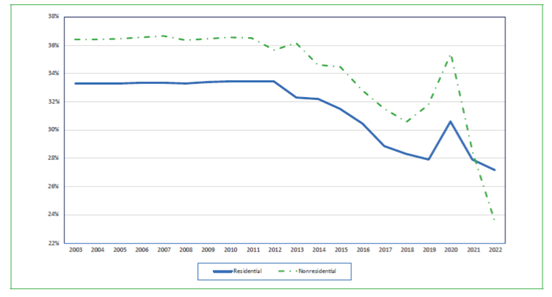
Continuing with residential construction, from 2003 up to 2012, the participation of the compensation of labor in gross value added remains with minor changes, averaging 33.6% (Graph 1). As from 2013, the share of labor in gross value added starts falling, reaching 27.8% in 2019. Its recovery of 30.6% in 2020, is followed by a fall below 28% in the following years.

Graph 1
Compensation of labor as a proportion of gva.* Residential and nonresidential construction. 2003-2022 (%)
*Gross value added adjusted for inflation.Source: Estimates based on Inegi.

Nonresidential construction averaged 36.4% from 2003 until 2013. This sector initiates its downfall in 2014 finding a respite of 31.8% in 2019. The year 2020 meant a recovery of 35.4. It reinitiates a downfall with a new bottom of 23.6 in 2022.

The brief boost of the share of labor compensation in both sectors is to be due to two factors. Value added fell due to the pandemic, while there was a tendency to preserve labor during adverse periods. This takes place considering the difficulty of finding an adequate workforce when a recovery takes place. It would imply that an element of labor hoarding has taken place.²³

Regarding the economy as a whole, the fall of labor compensation as a proportion of grow value added appears to be a general pattern in recent times. Stockhammer (2012) finds a falling trend among an array of high-income oecd countries using data from the beginning of 1970s until 2010.²⁴

Manyika et al. (2019) observe that the above proportion did drop in the United States from 63.3% in 2000 to 56.7% in 2016. Construction is quoted as one of the twelve sectors which explain much of this decline. In another paper for the United States, Abdih and Danninger (2017) find that several elements, i.e., change in capital labor ratios, foreign input intensity, automation of routine tasks as well as steep declines in unionization, play an important role for this decline.

Regarding Mexico, for Ibarra and Ros (2019), the fall in the compensation of labor as a share has been considerable.²⁵ They estimate a share of 28% in 2015, down from a rate close to 40% in mid-1970s. In searching for a cause, these authors note a fall in what they call union density and the establishing of a minimum wage policy. As an outcome, a higher profit share is attained according to these authors.

Following Joan Robinson (1923), a substantial amount of literature has emerged introducing the element of monopsony power to explain a profit share escalade.²⁶ Oseguera Sauri (2020), following Manning (2005), examines the existence of such power in the labor market, associated with the concentration of firms in Mexico. This study is done both in the formal and informal sectors of the economy, using the Herfindahl-Hirschman Index. A means to deter the concentration that she finds through a panel study, relies in the countervailing authority of the local antitrust commission.²⁷

4.6 Product wages and gross operational surplus as a share

To estimate the wages paid to labor considering his role in the production process, the price index of gross value added is utilized.²⁸ The product wage for labor in residential construction was 169.1 thousand pesos of 2022 for the 2003-2002 period, on average (Table 5). The lowest wage registered, i.e., 156.3 thousand pesos,²⁹ is similar to the average product wage of nonresidential workers. A difference of about one tenth in payment prevails among both groups of labor. The exception is regarding the maximum levels, as the gap between both falls.³⁰ The dispersion between both groups, measured by the coefficient of variation, is similar. In the case of residential construction, it is 0.049, slightly lower in comparison to its nonresidential counterpart (0.053).

Table 5

Product wages. Residential and nonresidential construction. 2003-2022 (Thousand of pesos of 2022)

Source: Estimates based on Inegi.

The statistical information available for gross operational surplus includes depreciation of capital. For residential and nonresidential construction, the percentage accrued to gross operational surplus is in the vicinity of two thirds. Such proportion is slightly above such share (67.9%) in the case of the former, and narrowly below (65.1%) the last one (Table 6).

Table 6

Residential and nonresidential construction. Gross operational surplus as a share of Gross value added. 2003-2022 (Percentage)

Source: Estimates based on Inegi.

The previous participation reached a maximum of three quarters of GDP (75.7%), for nonresidential construction. For its residential counterpart, such proportion rose beyond seventy percent. The lowest level of gross operational surplus as a share for residential construction surplus was close to two thirds (65.9%) and beyond three thirds (62.6%) regarding nonresidential construction.

Considering average wages,³¹ and gross operational surplus as a share, the relation of the former as a function of the last one regarding residential construction, is estimated as follows:

According to equation (5.1), there is a liaison between operational surplus as a share of GDP with a one year lag and average wages ³² In this case, a negative coefficient is being obtained (-1.25).³³ Therefore, an increase in the share of the above mentioned operational surplus, redounds in a substantial reduction in average wages.

Concerning nonresidential construction, the following estimate is obtained:

A link between the share of gross operational surplus as a share and average wages is registered regarding nonresidential construction. An elastic coefficient (-0.81) is obtained. In consequence, an increase in the operational surplus as a share has an opposite effect in average wages.

If it is assumed that value added is a given magnitude, it follows that an inverse relation between profits and wages woved apply. This last relation is expressed by Ricardo ([1821] 2001). It would be expected that average wages, in the previous model, would bear a negative relation with the gross operational surplus as a proxy for profits, placed as a share of gross value added.

4.7 Product wages and real wages

The examination of the compensation of labor as well as the corresponding estimate of average wages divided by job posts, has been systematically considered as an element of the production process until now. In this role, labor performs a role as a supplier of value added. In this respect, the compensation of labor as well as wages, have been adjusted for inflation with the gross value added deflator. Product wage refers to this process.

Labor also performs an additional role in the market, this time as a final consumer. In this role, labor becomes a demanding agent by spending his wages. It is by the consumer price index that these wages are adjusted for inflation. Hence, an estimate of what is known as real wage is obtained.

As the rate of inflation between gross value added in residential construction on the one hand, and the consumer price index on the other need not coincide, a wedge arises, to be estimated as follows:

The price index growth for residential output has outpaced the increase of the consumer price index. The ratio of the former with respect to the last one is of 2.0%, obtained from equation (6.1).³⁴ The price of the same average labor for the production process is higher as an element of production vis-à-vis its purchasing power as a final consumer. This difference runs in the benefit of labor as consumer. The compensation received is higher, considering the disbursement made in the purchase of labor power.

As far as nonresidential construction is concerned, the wedge between both price indices yieeds the following results:

The ratio between the gross value added deflator and the consumer price index exposes a growth of 2.1%. As in the case of residential construction, the product wage is higher that the real wage. It operates in the benefit of labor due to the lower increase in the price of final goods, in comparison to the price index of the value added that labor creates.

In neoclassical economics, the wedge is further identified as the gap between the marginal product of labor and the marginal rate of substitution of consumption for leisure (Shimer, 2009). A clarification is made by Kehoe et al. (2016), as the last one refers to a consumption labor-choice which happens to be static with the former.

Bosworth and Perry (1994), find that while real wages for the United States have remained below product wages, the former have been falling.³⁵ This pattern is being observed from the beginning of 1970s until the end of 1993. While these authors analyze this data along with productivity, the gap between these wages has been widening. Product wages have even exposed a modest decrement.

Conclusions

Key economic elements drawn from the economic accounts for the construction sector in Mexico are examined. The period under analysis is from 2003 to 2022. Gross output of residential construction has grown at a slower pace (1.9%), in comparison to nonresidential construction (2.6%). The gross output of the rest of the economy grew at an annual pace of 2.5% during this period.

Employment has interrupted its growth. The proxy for its measurement are job posts, as reported by the local statistical agency. They expose a contraction as from the second decade of this century. Employment in residential construction has fallen -7.1% from 2008 until 2018. Nonresidential construction faced a setback of -6.8% regarding employment from 2013 to 2018. In the first case, it did not recover from the local effect in the aftermath of the Great Recession. Residential construction contraction coincides with the presidential term of Enrique Peña Nieto. Reductions in the workforce of both sectors have continued. From 2019 to 2022, the deterioration persists, falling -12.3% and -9.6%, respectively, for residential and nonresidential construction.

The growth of intermediate consumption in both sectors of construction has been similar, i.e., 2.8% and 2.6% regarding residential and nonresidential components, respectively. Various shortfalls took place due to recessions including the Covid-19 pandemic, and a drop in housing finance. A recovery by nonresidential construction, growing at 12.4% annually in 2021 and 2022 is attested.

Employment in nonresidential construction exposes its capacity to grow at a lesser rate that the value of intermediate consumption, with an elasticity of 0.71. This coefficient contrasts with the corresponding one for its residential complement (1.26), suggesting an element of labor intensity in this last sector.

The compensation of labor as a share of gross value added was stable regarding residential construction from 2003 until 2012. This stability expands until 2013 regarding its nonresidential counterpart. While the average is 36.4% and 31.8% for the period as a whole, the compensation of labor share fell to 27.2% and 23.6% in 2022, respectively. The recession of 2020 for residential construction and 2019-2020 for the nonresidential sector, implies a recovery of this participation. This could be due to a fall in gross value added as well as labor hoarding, as the industry was envisaging an economic recovery. The erosion in labor shares appears to be a pattern on both national as well as international settings.

The product wage is estimated in relation to the share of operational surplus in value added. The elasticity for residential construction is -1.25, while -0.81 corresponds to the nonresidential sector, with a one year lag in both cases. A higher share of gross operational surplus appears to be attained at the expense of lower wages.

The product wage has been higher that the real wage for both construction sectors during the period of analysis. This is due to a lower growth of inflation of the consumer price index, in comparison to the index of gross value added in both sectors. As a result, real wages have not been deteriorated.

References

Abdih, Y. and Danninger, S. (2017). What explains the decline of the U.S. labor share of income? An analysis of state and industry data. Working Paper17(167). <https://www.imf.org/en/Publications/WP/Issues/2017/07/24/What-Explains-the-Decline-of-the-U-S-45086>.

Ashenfelter, O.C., Farber, H. and Ransom, M.R. (2010). Modern models of monopsony in labor markets: A brief survey. IZA Discussion Paper No. 4915. <https://docs.iza.org/dp4915.pdf>.

Banco de México. (1969). Cuentas nacionales y acervos de capital: consolidadas y por tipo de actividad económica, 1950-67. Mexico: Banco de México, Departamento de Estudios Económicos.

Banco de México. (2013). Informe trimestral, octubre-diciembre 2013. Mexico: Banco de México. <https://www.banxico.org.mx/publicaciones-y-prensa/informes-anuales/%7BEA277C6D-E723-7F50-4127-05EA6F2B6575%7D.pdf>.

Banco de México. (2014). Informe trimestral, julio-septiembre. México: Banco de México. <https://www.banxico.org.mx/publicaciones-y-prensa/informes-trimestrales/%7B897BB8E2-3D80-DF01-7B8C-F7D20A568BC3%7D.pdf>.

Bhaskar, V., Manning, A. and To, T. (2002). Oligopsony and monopsonistic competition in labor markets. Journal of Economic Perspectives, 16(2), 155-174. doi: 10.1257/0895330027300.

Boal, W.M. and Ransom, R. (1997). Monopsony in the labor market. Journal of Economic Literature35(1), 86-112. doi: 10.1257/aer.20200025.

Bosworth, B. and Perry, G.L. (1994). Productivity and wages: Is there a puzzle? Brookings Papers on Economic Activity, I, 317-344. <https://www.brookings.edu/wp-content/uploads/1994/01/1994a_bpea_bosworth_perry_shapiro.pdf>.

Cofece. (2015). Criterios técnicos para el cálculo y aplicación de un índice cuantitativo para medir la concentración del mercado. Mexico: Comisión Federal de Competencia Económica. <https://www.cofece.mx/wp-content/uploads/2017/11/criterios_tecnicos_para_medir_concentracin_del_mercado.pf>.

Coneval. (2023). Documento de análisis sobre la medición multidimensional de la pobreza, 2022. August. Mexico: Consejo Nacional de Evaluación de la Política de Desarrollo Social. <https://www.coneval.org.mx/Medicion/MP/Documents/MMP_2022/Documento_de_analisis_sobre_la_medicion_multidimensional_de_la_pobreza_2022.pdf>.

Colander, D. (2014). Gross output: a new revolutionary way to confuse students about measuring the economy. Eastern Economic Journal 40, 451-455. doi: 10.1057/eej.2014.39.

FAO. (1996). A system of economic accounts for food and agriculture. Rome: food and agriculture organization. <https://www.fao.org/3/W0010E/W0010E00.htm#Contents>.

Hall, R.E. (1991). Labor demand, labor supply and employment volatility. NBER Macroeconomics Annual, 6, 17-47 Chicago: University of Chicago Press. <https://www.jstor.org/stable/3585045>.

Hammermesh, D.S. (1993). Labor demand. Princeton: Princeton University Press.

Hicks, J. R. ([1932] 1963). The theory of wages. London: Palgrave Macmillan.

Hirsch, B., Elke, J.J. and Schnabel, C. (2018). Do employers have more monopsony power in slack labor markets? ILR Review71(3), 676-704. <https://www.jstor.org/stable/26956410>.

Hulten, C.R. (1992). Accounting for the wealth of nations: the net versus gross output controversy and its ramifications. Scandinavian Journal of Economics, Supplement. Proceedings of a Symposium on Productivity Concepts and Measurement Problems: Welfare, Quality and Productivity in the Service Industries, 94, S9-S24. doi: 10.2307/3440242.

Ibarra, C.A., and Ros, J. (2019). Why are workers getting a smaller share of the cake in Mexico? Blog. UNU Wider. Helsinki: United Nations University. <https://www.wider.unu.edu/publication/why-are-workers-getting-smaller-share-cake-mexico>.

Inegi (undated). Banco de Información Económica. Aguascalientes: Instituto Nacional de Estadística, Geografía e Informática <https://www.inegi.org.mx/app/ indicadores/?tm=0>.

Jorgenson, D.W., Landefeld, J.S. and Nordhaus, W.D. (2006). New architecture for the US national accounts. Chicago: NBER and University of Chicago Press.

Kehoe, P., Midrigan, V., Pastorino, E. (2016). Debt constraints and the labor wedge. American Economic Association Papers and Proceedings of the 128 Annual Meeting, 106(5), 548-553. <https://www.jstor.org/stable/43861080>.

Manning, A. (2005). Monopsony in motion: imperfect competition in labor markets. New Jersey: Princeton University Press.

Manyika, J., Mischke, J., Bughin, J., Woetzel, L., Krishnan, M. and Cudre, S. (2019). A new look at the declining labor share of income in the United States. Discussion Paper McKinsey Global Institute. <https://www.mckinsey.com/~/media/mckinsey/featured%20insights/employment%20and%20growth/a%20new%20look%20 at%20the%20declining%20labor%20share%20of%20income%20in%20 the%20united%20states/mgi-a-new-look-at-the-declining-labor-share-of-income-in-the-united-states.pdf>.

Marshall, A. (1890). Principles of economics, 8th edition. London: Palgrave Macmillan.

MacKinnon, J., Haug, A.A. and Michelis, L. (1999). Numerical Distribution Functions of Likelihood Ratio Tests for Cointegration. Journal of Applied Econometrics, 14, 563-577. <http://dx.doi.org/10.1002/(SICI)1099-1255(199909/10)14:5<563::AID-JAE530>3.0.CO;2-R>.

Mortensen, D.T. (1970). A theory of wage and employment dynamics (in Phelps, E.D., editor) Microeconomic foundations of employment and inflation theory. New York: Norton.

Munley, F. (1981). Wages, salaries, and the profit share: a reassessment of the evidence. Cambridge Journal of Economics, 5(2), 159-173. doi: 10.1093/oxfordjournals.cje.a035477.

NAICM (2016) Nuevo Aeropuerto Internacional de la Ciudad de México. Programa Estratégico/Institucional. Mexico: Grupo Aeroportuario de la Ciudad de México y Secretaría de Comunicaciones y Transportes <https://www.gacm.gob.mx/doc/pdf/naicm-interiores-vf.pdf>.

NAICS (2022) North American Industry Classification System. Washington: Excecutive Office of the President of the United States <https://www.census.gov/naics/reference_files_tools/2022_NAICS_Manual.pdf>.

Pigou, A.C. (1938). The economics of welfare. London: Macmillan.

NBER. (undated). Business cycle dating. Boston: National Bureau of Economic Research. <https://www.nber.org/research/business-cycle-dating>.

Oseguera Sauri, A.C. (2022). Concentración en el mercado laboral y su relación con los salarios en México. Estudios Económicos37(1), 45-102. doi: 10.24201/ee.v37i1.426.

Real Estate Market. (2014). Industria de la construcción profundizó contracción en 2013. Mexico: Real Estate Market. <https://realestatemarket.com.mx/noticias/infraestructura-y-construccion/13129-industria-de-la-construccion-profundizo-contraccion-en-2013.>.

Ricardo, D. ([1821] 2001). On the principles of political economy and taxation. Kitchener: Batoche Books. <https://socialsciences.mcmaster.ca/econ/ugcm/3ll3/ricardo/Principles.pdf>.

Robinson, J. (1923). The economics of imperfect competition. London: Macmillan.

Skousen, M. (1990). The structure of production. New York: New York University Press.

Skousen, M. (2017). Blocking progress in Austrian economics: A rejoinder. Procesos de Mercado. Revista Europea de Economía Política, 14(2), 143-172. doi: 10.52195/ pm.v17i1.14.

Stockhammer, E. (2012). Why have wage shares fallen? A panel analysis of the determinants of functional income distribution. ILO Conditions of Work and Employment Research SeriesNo.35, Geneva: International Labor Organization. <https://www.ilo.org/wcmsp5/groups/public/---ed_protect/---protrav/---travail/documents/publication/wcms_202352.pdf>.

World Bank. (undated). Gini Index-Mexico. Washington: The World Bank. <https://data.worldbank.org/indicator/SI.POV.GINI?locations=MX>.

Shimer, R. (2009). Convergence in macroeconomics: the labor wedge. American Economic Journal. Macroeconomics, 1(1), 280-297. doi: 10.1257/mac.1.1.280.

SNA. (2008). System of National Accounts. New York: United Nations et al. <https://unstats.un.org/unsd/nationalaccount/docs/SNA2008.pdf>.

Annex a. unit root tests

Table A.1.1

. Gross output growth rates

Table A.1.2

Employment growth rates

Table A.1.3.

Intermediate consumption growth rates

Table A.1.4

Labor compensation growth rates

Significance: ( )***: 99%; ( )**: 95%; ( )*: 90%.

Annex B. cointegration tests

Table B.2.1

Employment and the ratio of intermediate consumption and employment

Table B.2.2

Product wages and gross operational surplus as a share

Table B.2.3

Gross value added price and consumer price índices

Note. Trace test indicates no cointegration at the 0.05 level * denotes rejection of the hypothesis at the 0.05 level **MacKinnon-Haug-Michelis (1999) p-values

Notes