ARTICLES
Received: 14 August 2017
Accepted: 06 October 2017
DOI: 10.17230/ingciencia.13.26.3
Abstract: The numerical solution of transient stability problems is a key element for electrical power system operation. The classical model for multi-machine systems is defined as a set of non-linear differential equations for the rotor speed and the generator angle for each electrical machine, this mathematical model is usually known as the swing equations. This paper presents how to use direct Richardson extrapolation of several orders for the numerical solution of the swing equations and compares it with other commonly used implicit and explicit solvers such as Runge-Kutta, trapezoidal, Shampine and Radau methods. A numerical study on a simple three machine sys- tem is used to illustrate the performance and implementation of algebraic Richardson extrapolation coupled to several solution methods. Normally, the order of accuracy of any numerical solution can be increased when Richardson Extrapolation is used. A numerical example is provided for an electrical grid consisting of three machines and nine buses undergoing a disturbance. It is shown that in this case Richardson extrapolation effectively increases the order of accuracy of the explicit methods making them competitive with the implicit methods.
Key words: Power system transient stability, Richardson extrapolation, dynamic equations.
Resumen: La solución numérica de problemas de estabilidad transitoria es un elemento clave para la operación de sistemas eléctricos. El modelo clásico para sistemas multi-máquina se define como un conjunto de ecuaciones diferenciales no lineales para la velocidad del rotor y el ángulo del generador para cada máquina eléctrica, este modelo matemático se conoce generalmente como las ecuaciones de oscilación. Este artículo presenta la forma de utilizar la extrapolación directa de Richardson de varios órdenes para la solución numérica de las ecuaciones de oscilación y la compara con otros métodos implícitos y explícitos de uso común como los métodos RungeKutta, Trapezoidal, Shampine y Radau. Se presenta un estudio numérico sobre un sistema simple de tres máquinas para ilustrar el desempeño y la implementación algebráica de la extrapolación de Richardson. El orden de exactitud de cualquier solución numérica puede aumentarse cuando se utiliza la extrapolación de Richardson. Se proporciona un ejemplo numérico para una red eléctrica que consta de tres máquinas y nueve buses que sufren una perturbación. Se demuestra que en este caso la extrapolación de Richardson aumenta efectivamente el orden de exactitud de los métodos explícitos haciéndolos competitivos con los métodos implícitos.
Palabras clave: Estabilidad transitoria de sistemas de potencia, extrapolación de Richardson, ecuaciones dinámicas..
1 Introduction
The transient stability analysis in electrical grids is important to evaluate the effects of disturbances in rotors in power systems operation, security, and maintenance. Several researchers have applied numerical integration methods for solving the classical swing equations 1,2,3 to obtain the behavior of the power angles and the rotational speeds in the time domain. Classical numerical methods both implicit and explicit 4,5,6,7 can be employed to find accurate results because numerical integration of the non linear differential equations is performed. The transient stability analysis (TSA) is very important for the design of electric power systems because it allows to determine the system’s ability to withstand large disturbances and to transition to a normal operating condition. These disturbances can be faults such as: short and open circuits on a transmission line, loss of a generator, loss of a load, gain of load or loss of a portion of transmission network 8,9,10. For multi-machine stability analysis, the condition of the system and grid configuration before and after the disturbance, must be known. Therefore, two preliminary stages are needed before the transient study: the pre-fault conditions for the system which are calculated by a load flow balance, then the representation of the grid before the fault is modified to take into account the conditions during and after the failure 9. Regular numerical simulations are also important during planning stages to gain knowledge of the system. Yet, even a well designed system may face transient instability issues 11. The application and assesment of innovative numerical methods for solving transient stability situations is currently of interest because it allows the development of high accuracy computational packages and it may also have additional advantages for research and academical purposes. The solution of TSA problems involves two main stages, the network analysis and the dynamic model solution 2.
The network analysis includes the power load solution for determining the initial bus angles and voltages and the computation of the reduced admittance matrix. The dynamic model solves the transient differential equations for each machine in the system yielding the values of the angular velocities and the angles. These variables are important in studies of transient stability enhancement control 12, 13, 14. The set of differential equations, which can be highly nonlinear depending on the machine model used, are solved by a numerical method, for each time step.
In this paper the combination of the Richardson extrapolation 15 with different numerical methods is studied to determine its advantages respect to tradditional methods, such as the trapezoidal integration commonly used in power system dynamic equations 16. Initially, in this work the classical wing equations for rotor dynamics are solved with several numerical methods both explicit and implicit such as euler, trapezoidal (semi-implicit), Runge kutta, Shampine 4 and Radau 17. Then, the above methods are combined with Richardson extrapolation to evaluate and compare the accuracy and the order improvement of the resulting combined schemes.
2 Power system model
A multi-machine system has several synchronous generators which can be modelled by two differential nonlinear equations. This model is called the classical model or swing equations represented as follows:
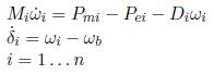 (1)
(1)where n is the number of rotor machines, δ i is the rotor angle of the i − th machine, ω i is the angular speed, ω b is the base velocity of the system, M i is the moment of inertia, D i is the damping coefficient and P mi and P ei are the mechanical and electrical power respectively. The rotor angle is constant when the machines are in steady state when ω i = ω b that is also the velocity initial condition in the pre-fault state. The initial conditions of generator rotor angles and emf (E) are also obtained from the system prefault conditions [18]. After an electrical disturbance the rotor angle changes from a constant value to another after the transient stage, assuming that stability is maintained.
The electrical power P e,i of machine i is calculated from
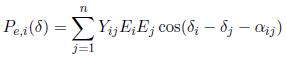 (2)
(2)where Y ij are the entries of a reduced admittance matrix 19, E i is the i-th voltage behind the transient reactance, and α ij are the admittance phase angles. Note that equations (1) and (2) can be seen either as a coupled algebraic-differential system or as a nonlinear differential system when equation (2) is subtituted in (1). The presented formulation allows reducing the number of unknown variables, because bus voltages as well as the equations of current injections at network buses are not needed 18, 3. During the stability study, the assumptions made are 16, 20, 21: Mechanical power input is constant, damping is neglected, constant voltage behind the transient reactance model of the synchronous machine is valid, the mechanical rotor angle is assumed to be equal to the angle of the voltage behind the transient reactance, and the loads are represented by passive impedances.
An electrical network with n nodes from the standpoint of the generator terminals, has an admittance matrix  defined by:
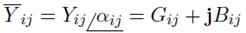 (3)
(3)To calculate the above matrix several steps are usually needed. First, the equivalent impedances or admittances are connected between the load buses and the reference node. Also, calculation of the fault impedances is added, and the admittance matrix is modified for each switching condition. Secondly, equivalent admittances are obtained for each impedance element. Finally, elements of the Y matrix are obtained as follows: Y ii is the sum of all the admittances connected to node i, and Y ij is the negative of the admittance between node i and j. After the admittance matrix has been obtained for the original network, it can be reduced by eliminating all but those corresponding to generators. This procedure known as Kron reduction 22 can be achieved by row-column operations considering that all the nodes have net zero current except for the internal generator ones. Thus, a reduced system is obtained as shown below
 (4)
(4)where
 (5)
(5)Now the system in (4) is partitioned to get
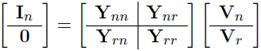 (6)
(6)where n indicates the generator nodes and r is used for the remaining nodes. Now, expanding (6) and eliminating V r , the result is
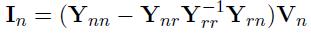 (7)
(7)The reduced matrix 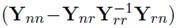 only contains the coefficients that correspond to the generator nodes. The network simplified equation represented in (7) is a convenient analytical technique that can be used when the loads are treated as constant impedances, this elimination procedure can be applied only to those nodes with zero current. The Kron reduction is the most important step prior to the transient solution. Also, it is a standard tool to obtain stationary and dynamically-equivalent reduced models for power flow studies, or in the reduction of differential-algebraic systems to lower dimensional dynamic models of power networks 22.
3 Richardson extrapolation combined with the numerical solution methods
The numerical solution of the power system equations can be improved by means of Richardson extrapolation which is an efficient technique for enhancing the accuracy of integration schemes 15. To explain how Richardson extrapolation can be applied to the solution of the swing equations, let consider A(h) the numerical solution of the system (1) which depends on the step size h, thus
 (8)
(8)where a 0 is the solution that is being sought as the time step h approaches 0, i.e. A(h) → a 0, and O(h p+n )is the Landau symbol representing the truncation error terms of order p + n an higher. Substituting different step sizes h,h/2,h/4,etc. into (8), the following system of equations can be assembled,
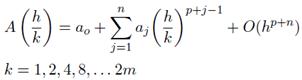 (9)
(9)For example, if only the first two terms of the series (8) are taken, the numerical solution method of order p would be written as
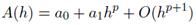 (10)
(10)and the following system is obtained
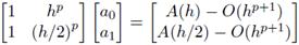 (11)
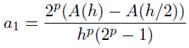
(11)solving the system of equations yields,
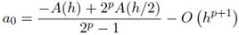 (12)
(12)
 (13)
(13)where it is clear that the new approximation a 0, being of order p + 1, will be more accurate than both A(h) and A(h/2) 15. Equation (12) shows that Richardson extrapolation can be used to accelerate the convergence of a numerical method. If a numerical method for solving a differential equation like Runge-Kutta, trapezoidal, etc. converges as O(h p ), the error can be reduced by a factor of h to produce a technique that converges as O(h p+1 ), and this can be used iteratively to produce other approximations that converge at any chosen rate. Hence, Richardson extrapolation can be used to obtain a higher order approximation for the dynamic equations (1) by increasing the order of any numerical method used to solved them. Note that the approximation a 0 given in equation (12) involves two numerical solutions, one with the total time step A(h), and another one with two shorter steps of size h/2 used to obtain the second numerical approximation A(h/2) at the end of the interval. Higher order Richardson extrapolation formulae can be deduced from equations (8) and (9) if more terms of the series (8) are retained. For example, if three terms of the series are used, the following system is obtained
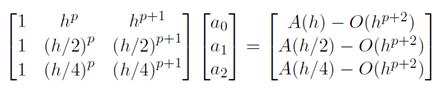 (14)
(14)which leads to he new approximation
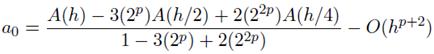 (15)
(15)Similarly, if four terms of (8) are employed, a system of four equations is obtained whose solution gives the following higher order approximation
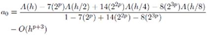 (16)
(16)It can be seen that to obtain the higher order approximations defined in equations (15)-(16), the problem in each time interval must be solved several times but using different time step sizes. The first solution A(h) in one step with length h, the solution A(h/2) obtained with two smaller steps of size h/2, A(h/4) with four h/4 size steps, A(h/8) with eight h size steps and so on. Although this procedure increases the computational cost, it also improves the order of accuracy. Thus, if for example Runge Kutta method of order p = 2 were used to obtain the approximations A(h) and A(h/2), equation (12) would give a higher order solution of order p + 1 = 3. Likewise, if the mentioned Runge Kutta method were used to obtain the approximate solutions A(h), A(h/2), A(h/4) and A(h/8), equation (16) would define a new approximation of order p + 3 = 5 higher than the original Runge Kutta used. Some stability theorems about the combination of different solution methods with Richardson extrapolation are discussed in 15. A short discussion of the solution methods used in the present work that can be combined with Richardson extrapolation is presented in the following section in order to understand the obtained results.
4 Overview of numerical solution methods for electrical power systems
There are several methods for the approximate solution of the swing equations such as: Euler’s method, semi-implicit Euler method (trapezoidal), collocation, Runge Kutta, shampine, Radeau, among many more. Some of these methods are classified as implicit or explicit, in fact some methods like Runge-Kutta can be stated as either of these categories. Furthermore, the solution schemes may be classified according to the kind of problem i.e. there are special techniques for non-linear ordinary differential equations (ODE), and other for algebraic-differential systems. All of the mentioned methods are essentially iterative or sequential procedures that allow to calculate the power angle δ and the rotor velocity ω as a function of time, and to determine whether or not the system is stable.
4.1 Euler method
It is the most basic explicit method for numerical solution of ordinary differential equations and it can also be regarded as the simplest first order Runge-Kutta method. Most solution methods require the ODE to be written in the form
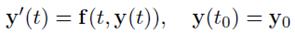 (17)
(17)for the case of the stability equations (1) the function vector is defined as
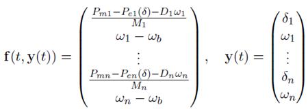 (18)
(18)and the Euler method defines the forward step
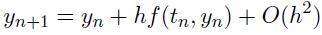 (19)
(19)where h is the time step size. The Euler method can be numerically unstable depending on the step size, especially for stiff equations. The implicit variant of the Euler method is defined as
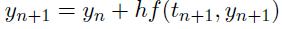 (20)
(20)and it can clearly be observed that in this case the equations are non-linear and they need to be solved by Newton method or other similar iterative techniques to obtain the value of y n+1 .
4.2 Semi-implicit methods
The simplest semi implicit method is the trapezoidal integration rule 23 that is based on Euler method by averaging the derivative values,
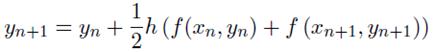 (21)
(21)note that this method requeries non-linear iteration to find y n+1 value.
A semi-implicit method for the solution of the differential-algebraic equations (DAE) describing transient stability models, is proposed by Milano [3]. DAE systems are formulated as
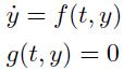 (22)
(22)As stated in equations (1) and (2), the function g(t, y) defines the electrical power P ei . This formulation coupled with an implicit integration scheme has two advantages when compared to the conventional explicit formulation: it reduces the computational burden and increases the sparsity of the Jacobian matrix of the system.
4.3 Shampine implicit method
An implicit method for the solution of sets of first order differential equations was developed by Shampine 4. In this method the problem must be formulated as
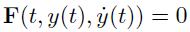 (23)
(23)The mentioned method is based on the Lagrangian form of polynomial interpolation and it is applied to improve the MATLAB built-in solvers (ode15i) 24. Furthermore, Shampine algorithm is usually considered as embedded method that produces an estimate of the local truncation error and as a result allows to control the error with adaptive stepsize.
4.4 Runge-Kutta methods
There are several families of Runge-Kutta methods (RK), both explicit and implicit and they may also have different orders. For example, the fourth order explicit RK methods is
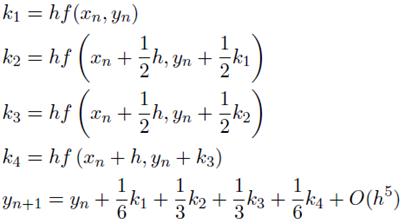 (24)
(24)The explicit RK methods can be generalized as
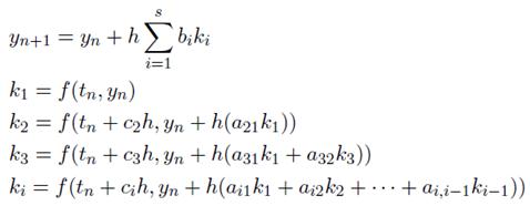 (25)
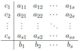
(25)The coefficients can be arranged in the following tableau form 25,
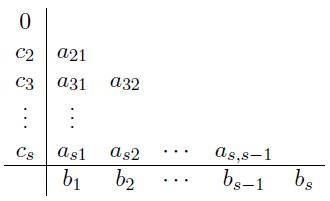 (26)
(26)The explicit RK methods have a bounded stability region [26] specially when stiff or discontinous problems are concerned. The inestability issues motivate the development of implicit RK methods 26 which are usually expressed as,
 (27)
(27)with corresponding coefficient matrix,
 (28)
(28)Equations (27)-(28) are non linear and need to be solved to find the values of the k i coefficients.
4.5 Radau methods
These are fully implicit methods where the coefficient matrix (28) may have any structure, and they are usually appropiate for stiff systems. Radau methods are A-stable 5 but expensive to implement like all the implicit methods that need some sort of Newton iteration 17, 6, 5. Some alternatives have been proposed to reduce the computational cost that are usually based on approximate Jacobian matrix and dimensionality reduction 17.
5 Numerical results
In this section the proposed Richardson method of several orders equations (13),(15) and (16), will be used to obtain the numerical solution for the IEEE 3-machine 9-bus system under a three-phase fault. The base MVA and system frequency are considered to be 100 MVA and 60 Hz, respectively.
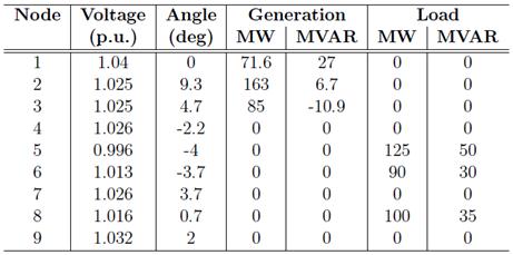
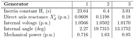
Numerical experiments using different solution methods combined with Richardson extrapolation are presented to compare their performance. In the analyzed power network, Generator 1 is a hydro electric plant, while 2 and 3 are steam generators. Tables 1-2 show the load flow data needed for the solution, the electric power computation and the initial conditions. The simulated disturbance initiating the transient stage occurs near bus 7 at the end of line 5-7. The fault is cleared in 5 cycles (0.083 s) by opening line 5-7.
Load flow for IEEE 3-machine 9-bus system
Generator internal voltages and their initial angles
The steps for the numerical experiments are the following:
-
After modeling the network, a load flow analysis is performed to obtain the initial bus voltages, the initial machine input and the power output.
-
Compute the internal machine voltages
-
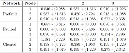
Compute the prefault system admittance matrix Y pre and its Kron reduction as in (7) (Table 3)
-
At the initial time t = 0 set the faulted bus voltages to zero
-
Compute the faulted system admittance matrix Y fault by setting to zero the rows and columns of the initial matrix Y pre that correspond to the disturbed line. Also, the fault impedance is added as requiered and the admittance matrix is determined for each switching condition. Calculate the Kron reduction for Y fault .
-
Compute the post-fault system admittance matrix Y post and its kron reduction. Solve the differential equations by using different solvers alone and combined with Richardson extrapolation to compare the results.
Reduced admittance matrices
A computer code was designed and implemented in MATLAB environment for the numerical solution of the transient problem that describe the power network dynamics during a disturbance. The main purpose of the program is to show how Richardson extrapolation can be used togetherwith both explicit and implicit solution methods to improve their order of accuracy. In Figure 1 the rotor angle variation with time is shown for each machine.
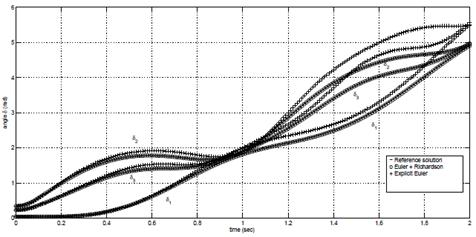
Figure 1
Rotor angle versus time
This figure compares the results obtained by Euler explicit method with constant step width and by the Euler method improved by Richardson extrapolation with the reference solution given by DIGSILENT 27 and shown by 9. It is noticeable that the explicit Euler method with error order O(h 2) is improved by Richardson equation (16) with order O(h 5) according to what was explained in section 3, and the same trend can be observed for the angular velocity depicted in Figure 2.
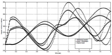
Figure 2:
Angular velocity versus time
A plot of the angle differences of the machines in the system, δ 2 −δ 1 and δ 3 − δ 1 is shown in Figure 3, where it can be seen again that Richardson method considerably improves an explicit method such as Euler. Note that the solution is carried out in two swings to show that relative rotor angles swing together with respect to the simulation time and therefore the system is stable. A suitable criterion for stability is that if the rotor angle differences reach maximum values and then decrease, the system is stable 21. However, if any of the angle differences increases indefinitely the system is considered unstable because at least one machine would be out of synchronism.
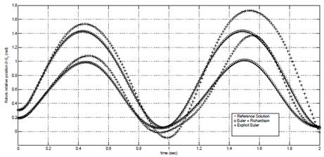
Figure 3:
Variation of angle differences δ2 − δ1 and δ3 − δ1
Figure 4 and 5 show the rotor angle and velocity mean errors respectively. These figures were obtained with different solution methods like explicit Euler, Runge-Kutta of order 2 (RK2), Semi-implicit trapezoidal, Radau methods of orders 3 and 5, Shampine implicit method, Euler improved by Richardson and trapezoidal improved by Richardson. It can be seen, in both figures, that the methods improved by Richardson extrapolation surpass in accuracy all the other methods with constant step width, with the exception of the Shampine fully implicit method that uses adaptive variable step size. The mean errors for the three generators are defined as
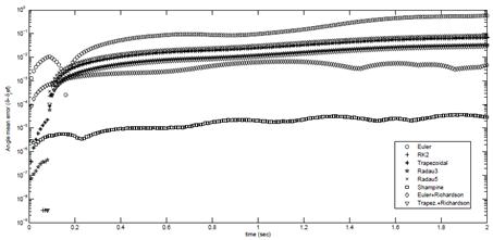
Figure 4:
Rotor angle mean error δ − δ ref
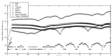
Figure 5:
Rotor velocity mean error ω − ω ref
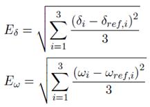 (29)
(29)where δref,i,ωref,i represent the reference solutions already mentioned. Note that the mean errors stay fairly uniform after the fault has been cleared.
The comparison of the absolute errors for different numerical solutions is shown in Figure 6 and 7 for the angle and velocity respectively. The total absolute errors for the three generators are defined as
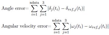 (30)
(30)where ndata is the total number of time values or steps in the numerical solution. Figure 4 and 5 present the comparison of some explicit and implicit methods, methods of different orders and the effect of Richardson extrapolation applied to some of these methods. Low order explicit methods such as Euler, which has order 1 i.e. O(h2), yield higher errors than other explicit methods of higher order or the implicit methods. Note that the overall error is lower when the solution is calculated by methods of higher order, or when implicit or semi-implicit methods are used, or when Richardson extrapolation is combined with any method to improve its accuracy. Most of the methods presented in Figures 6 and 7 have constant time step except the Shampine method which includes adaptive control of error with variable step size and therefore its associated error is very small. Additionally, when Richardson extrapolation is combined with an integration method the results are noticeably improved and thus Richardson extrapolation can make explicit methods comparable with implicit and multi-step methods. In short, there are several alternatives to lower the numerical error: To use shorter integration step, to use adaptive step error control, to use high order methods either explicit or implicit and to improve the methods by coupling them with Richardson extrapolation. Also, the previous alternatives could be used combined among them to obtain highly accurate solutions.
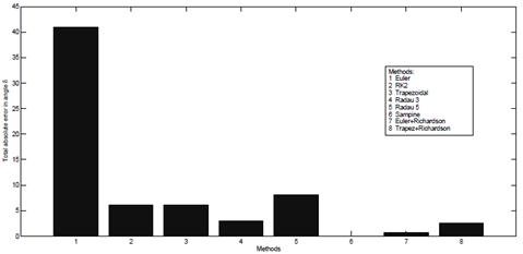
Figure 6:
Overall angle error comparison for different methods
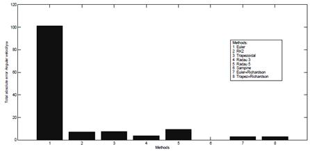
Figure 7:
Overall velocity error comparison for different methods
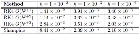
Usually, in most numerical methods as the step size becomes smaller, the less error is obtained. This behavior is observed in Table (4) where the fourth order Runke Kutta method combined with Richardson extrapolation, and the Shampine method were used with different step sizes to approximate the solution of equation (1). For the Runge Kutta method the step size value was kept constant on the entire integration interval, while due to its adaptive nature, in the Shampine method the step value h refers to the maximum initial step size allowed. The order of the Runge Kutta method was increased by combining it with Richardson extrapolation according to formulae (13),(15) and (16), hence theoretically the combined methods would have errors of order O(h6),O(h7) and O(h8) respectively. For example, it can be seen, for an explicit method like Runge Kutta of fourth order (RK4) combined with Richardson of error order O(hp+1), the mean error goes from 1.41 × 10⁻² to 3.40 × 10⁻³ for step sizes h = 1 × 10⁻² and h = 1 × 10⁻⁴ respectively. Hence, the reduction of the step size produced almost 4 times less error. Similar error reduction can be accomplished if the Richardson order increases from O(hp+1) to O(hp+3) with a constant step of h = 1 × 10⁻², the error value 1.41 × 10⁻² lowers to 2.84 × 10⁻³ which means a reduction almost by a factor of 5. Similar results can be observed in the other rows and columns of Table 4 that illustrates how, from an accuracy standpoint, an explicit method improved by Richardson extrapolation can be made competitive with other more sophisticated implicit methods such as Shampine.
Effect of the step size on several solution methods
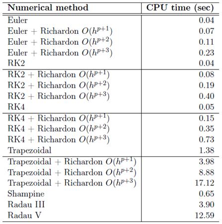
The error reduction effect associated with Richardson method can be confirmed in Figure 8. It can be seen that when the order of the Richardson extrapolation is higher the error becomes smaller regardeless of the integration method being explicit or implicit. However, this improvement in accuracy comes at the expense of computational time as presented in Table 5, which shows that the cpu time becomes higher either when the order of the integration method is high or the order of Richardson is increased. The lower order methods need few operations, therefore their CPU time is lower. In contrast, implicit methods take longer not only because they need more operations to advance one step, but also because they require Newton iterations to account for their inherent non-linearity. Note that when the Richardson order is increased, the CPU time is doubled. However, it can be seen that a lower order explicit method combined with Richardson becomes comparable in time and accuracy with a higher order implicit method. For example, an Euler method with Richardson extrapolation of error order O(hp+3) takes 0.23 seconds, while the trapezoidal spends 1.38 seconds to achieve less accuracy than the improved Euler method as was shown in Figure 6 and 7.
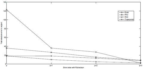
Figure 8
Effect of increasing the order of Richardson extrapolation
CPU time for the numerical solution by different methods
6 Conclusions
This paper presented the numerical solution of a transient stability problem for the IEEE 3-machine 9-bus system using different numerical methods. The integration methods are compared, and the effect of combining them with Richardson extrapolation of several orders is analyzed. The obtained numerical results are in agreement with a reference solution calculated by software Digsilent and also presented in several literature references. The proposed Richardson extrapolation schemes of several orders are presented based on an algebraic approach rather than in the conventional recursion method. It was found that Richardson approach really improves the explicit methods making them competitive with the implicit ones. Also, although Richardson method increases the computational time when increasing the order of the approximation, the solution time of the explicit methods improved by Richardson stays well below their implicit counterparts, while the accuracy of the solution improves considerably
References
1. M. Watanabe, Y. Mitani, and K. Tsuji, “A numerical method to evaluate power system global stability determined by limit cycle,” IEEE Transactions on Power Systems, vol. 19, no. 4, pp. 1925-1934, Nov 2004. 67
2. J. H. Chow and K. W. Cheung, “A toolbox for power system dynamics and control engineering education and research,” IEEE Transactions on Power Systems , vol. 7, no. 4, pp. 1559-1564, Nov 1992. 67
3. F. Milano, “Semi-implicit formulation of differential-algebraic equations for transient stability analysis,” IEEE Transactions on Power Systems , vol. PP, no. 99, pp. 1-10, 2016. 67, 69, 74
4. L. Shampine, “Solving 0 = f(t, y(t), y(t)) in matlab,” Numerical Mathematics, vol. 10, pp. 291 - 310, 2002. 67, 68, 74
5. E. Hairer and G. Wanner, “Stiff differential equations solved by radau methods,” Journal of Computational and Applied Mathematics, vol. 111, no. 1002, pp. 93 - 111, 1999. (Online). Available: http://www.sciencedirect.com/science/article/pii/S037704279900134X 67, 76
6. A. Aubry and P. Chartier, “On the structure of errors for radau ia methods applied to index-2 daes,” Applied Numerical Mathematics , vol. 22, no. 1, pp. 23 - 34, 1996. [Online]. Available: http://www.sciencedirect.com/science/article/pii/S0168927496000232 67, 76
7. K. S. Shetye, T. J. Overbye, S. Mohapatra, R. Xu, J. F. Gronquist, and T. L. Doern, “Systematic determination of discrepancies across transient stability software packages,” IEEE Transactions on Power Systems , vol. 31, no. 1, pp. 432-441, Jan 2016. 67
8. A. Singh and S. Parida, “A multiple strategic evaluation for fault detection in electrical power system,” International Journal of Electrical Power & Energy Systems, vol. 48, pp. 21 - 30, 2013. [Online]. Available: http://www.sciencedirect.com/science/article/pii/S0142061512006862 67
9. A. Paul M. Anderson, Power System Control and Stability. Wiley, 2002. 67, 79
10. W. D. Stevenson Jr. and J. J. Grainger, Power system analysis. McGraw-Hill, 1994. 67
11. P. K. Iyambo and R. Tzoneva, “Transient stability analysis of the ieee 14-bus electric power system,” in AFRICON 2007, Sept 2007, pp. 1-9. 67
12. A. Farraj, E. Hammad, and D. Kundur, “A cyber-physical control framework for transient stability in smart grids,” IEEE Transactions on Smart Grid, vol. PP, no. 99, pp. 1-10, 2016. 67
13. C. Rehtanz and X. Guillaud , “Real-time and co-simulations for the development of power system monitoring, control and protection,” in 2016 Power Systems Computation Conference (PSCC), June 2016 , pp. 1-20. 67
14. S. Teleke, “Modeling and comparison of synchronous condenser and svc,” Master’s thesis, Chalmers University Of Technology, 2006. 67
15. Z. Zlatev, K. Georgiev, and I. Dimov, “Studying absolute stability properties of the richardson extrapolation combined with explicit runge kutta methods,” Computers & Mathematics with Applications, vol. 67, no. 12, pp. 2294 - 2307, 2014, 67, 70, 71, 72
16. Y. C Evrenoso~glu and H. Dag, “Detailed model for power system transient stability analysis,” Journal of Engineering & Computer Science IJECS-IJENS , vol. 13, no. 2, pp. 1 - 5, 2012. 67, 69
17. D. XIE, “A new numerical algorithm for efficiently implementing implicit runge-kutta methods,” Department of Mathematical Sciences. University of Wisconsin, Milwaukee, Wisconsin, USA, pp. 1 - 17, 2009. 68, 76
18. R. Zarate-Minano, T. V. Cutsem, F. Milano, and A. J. Conejo, “Securing transient stability using time-domain simulations within an optimal power flow,” IEEE Transactions on Power Systems , vol. 25, no. 1, pp. 243-253, Feb 2010. 68, 69
19. S. Sharma, S. Kulkarni, A. Maksud, S. R. Wagh, and N. M. Singh, “Transient stability assessment and synchronization of multimachine power system using kuramoto model,” in North American Power Symposium (NAPS), 2013, Sept 2013, pp. 1-6. 68
20. S. Ekinci and A. Demiroren, “Transient stability simulation of multi-machine power systems using simulink,” Electrical & Electronics Engineering, vol. 15, no. 2, pp. 1 - 8, 2015. 69
21. Q. M. R. M. A. Salam, M. A. Rashid and M. Rizon, “Transient stability analysis of a three-machine nine bus power system network,” Engineering Letters, vol. 22, no. 1, pp. 1 - 7, 2014. 69, 80
22. F. Dorfler and F. Bullo, “Kron reduction of graphs with applications to electrical networks,” IEEE Transactions on Circuits and Systems I: Regular Papers, vol. 60, no. 1, pp. 150-163, Jan 2013. 69, 70
23. W. H. Press, S. A. Teukolsky, W. T. Vetterling, and B. P. Flannery, Numerical Recipes 3rd Edition: The Art of Scientific Computing, 3rd ed. New York, NY, USA: Cambridge University Press, 2007. 74, 75
24. MATLAB, version R2015. Natick, Massachusetts: The MathWorks Inc., 2015. 74
25. J. C. Butcher, “Implicit runge-kutta processes,” Mathematics of Computation, vol. 18, no. 85, pp. 50-64, 1964. (Online). Available: http://www.jstor.org/stable/2003405 75
26. E. Süli, D. F. Mayers, An Introduction to Numerical Analysis. Cambridge University Press, 2003. 75, 76
27. Digsilent powerfactory. (Online). Available: http://www.digsilent.de/ 79
