INTRODUCTION

Financial market volatility is a very important phenomenon in the global economy due to its significant impact on investment decisions, monetary policy, and economic stability (Mensi et al., 2016). The ASEAN-5 region, which consists of Indonesia, Malaysia, the Philippines, Singapore, and Thailand, comprises countries with high economic, social, and political diversity. These nations, nevertheless, have strong ties in commerce, investment, and economic reliance (Winantyo et al., 2008). Economic contacts among ASEAN-5 nations are getting deeper as globalization proceeds, establishing close links between their financial markets (Owen et al., 2019).

Moreover, ASEAN-5 amply illustrates how financial and economic integration could affect the stability of regional and world markets. These nations serve as part of more extensive economic networks linked by trade, investment, and capital movements, in addition to being independent economic entities. Long acknowledged as a major regional financial center, Singapore helps connect markets in ASEAN with worldwide capital markets (Oetomo et al., 2016). Conversely, Indonesia’s sizable and active home market significantly boosts the regional economy by means of both domestic consumption and international investment. Significant market volatility in the ASEAN-5 area can be brought about by changes in monetary and fiscal policy, as well as political instability and external events such as the global financial crisis (Munthe, 2017). The 2008 global financial crisis demonstrated how rapidly economic shocks in one area of the world may travel to other financial markets, thereby triggering a domino effect that influences global economic stability (Acharya et al., 2011; Mensi et al., 2016). This emphasizes the need to understand how risk and market volatility could be distributed among linked nations (Zhou et al., 2021).

The financial markets in ASEAN-5 exhibit significant complexity and volatility, influenced by both economic and non-financial factors. Macroeconomic factors, including fiscal and monetary policies, significantly influence these markets, alongside the global economic context (Darinda & Permana, 2019). Investors adjust their portfolios in response to alterations in the cost of capital and expectations regarding economic growth. For instance, fluctuations in central bank interest rates can lead to rapid and significant shifts in market volatility (Bodea & Hicks, 2015). Increases in analogous volatility may also arise from fiscal policies and unforeseen global events, such as geopolitical issues or natural disasters (Adekoya & Oliyide, 2021).

Additionally, non-financial factors contributing to uncertainty and exacerbating market instability include geopolitical tensions, such as those in the South China Sea, and political events like elections (Liu et al., 2023). Investor sentiment, characterized by panic or excessive optimism, further amplifies these fluctuations. Understanding volatility spillovers in ASEAN-5 markets is essential for informing systemic risk management strategies (Purbasari, 2019). A comprehensive understanding of political and economic factors influencing volatility in ASEAN-5 financial markets enables market participants to anticipate changes and formulate adaptable, informed investment strategies that are more resilient to regional and global market fluctuations.

Furthermore, the use of the value at risk (VaR) method is key in measuring and managing market risk in the ASEAN-5 financial markets (Boonyakunakorn et al., 2019). By examining the probability distribution of possible losses that could occur in a given period, VaR offers a strong method to assess potential losses in investment portfolios (Tsay, 2005). Using VaR helps investors and portfolio managers in the ASEAN-5 environment - where market risks can vary greatly between nations and sectors - to spot possible hazards and more effectively allocate resources (Ahadiat & Kesumah, 2021). VaR facilitates the understanding of the risk interrelationships between financial markets in ASEAN-5 since it allows one to project the degree of losses that might arise in circumstances where market volatility or turbulence rises rapidly (Bautista & Mora, 2021). VaR also lets portfolio managers modify their investment plans based on the desired risk profile, thereby enabling the attainment of long-term investment targets (Engle & Manganelli, 2004). Thus, among the complex and changing market dynamics in ASEAN-5 financial markets, we employ VaR measurement to offer a strong tool for investors and portfolio managers to properly control risk and maximize portfolio performance.

This study is grounded in systemic risk theory, which posits that financial interdependence amplifies vulnerability to external shocks. ASEAN-5 markets serve as a case study to illustrate how interconnected markets propagate volatility, creating systemic risks that challenge traditional diversification strategies. By quantifying these risks through VaR, this research bridges theoretical insights with practical applications for investors and regulators. This study presents a framework that allows market participants to adjust strategies in response to evolving conditions by modeling spillover effects and quantifying risk through VaR (Boonyakunakorn et al., 2019).

This research introduces a novel application of the VaR approach to assess potential losses in ASEAN-5 markets considering endogeneity. Changes in endogeneity are crucial to avoid biased outcomes in volatility analysis due to their interdependence. This study employs lagged variables and control measures, alongside instrument-based strategies, to mitigate endogeneity, thereby enhancing the precision of risk spillover estimations and affirming VaR as an effective instrument in these interconnected markets (Engle & Manganelli, 2004; Liu et al., 2022).

Consequently, while the existing literature has explored volatility spillovers and their implications, this study extends these discussions by incorporating the VaR framework to assess risk exposure in ASEAN-5 markets during periods of extreme disruption. Drawing on systemic risk theory, the study provides a nuanced understanding of interconnected financial systems and the propagation of shocks. By focusing on the ASEAN-5 region, this research contributes to ongoing debates on market integration and the effectiveness of diversification strategies, thereby improving regional market stability and fostering sustainable development. For this reason, we build the research question of how volatility is transmitted between ASEAN-5 countries and how the level of risk can be measured using the VaR approach in each ASEAN-5 country.

LITERATURE REVIEWS

Economic integration and volatility spillover in emerging markets

Economic integration can be interpreted as a process in which a group of countries carries out commercial or trade policies that reduce trade barriers only between certain parties to increase prosperity (Winantyo et al., 2008). The liberalization of trade and investment reflects global economic integration, facilitating interconnected capital markets. That integration enables investors to diversify portfolios without national barriers, resulting in synchronized market indices and co-movements of asset prices (Horvath & Petrovski, 2013; Jovanović & Lipsey, 2006).

Furthermore, a number of previous studies have observed volatility spillovers in emerging markets like ASEAN-5 countries. Darinda and Permana (2019) explored volatility transmission patterns in the financial markets of ASEAN-5 countries using proxy variables for Brent-oil prices as indicators measuring macro shocks, and exchange rate variables as proxies for the fundamental conditions of a country. By applying the VAR and GARCH (1,1)-BEKK models, this research found that all independent variables have significant volatility transmission to the stock market in ASEAN-5 countries, and there are differences in the volatility transmission patterns of the Malaysian stock market (KLCI), Thai stock market (SETI), and Philippine stock market (PSEI).

Similarly, Sumani and Saadah (2019) investigated the phenomenon of stock price volatility transmission in each ASEAN-5 country stock market. The findings showed that shocks occurring in the stock markets of Singapore, Malaysia, Thailand, and the Philippines are transmitted to the Indonesian stock market with an asymmetric pattern, as revealed by the EGARCH model test. The latest study by Danila (2023), regarding co-movement testing and spillover volatility between the stock markets of ASEAN countries and GCC (Gulf Cooperation Council) countries, found that sharia and conventional stock indices respond to each other in each country. Hence, these studies underscore the interconnectedness of emerging markets and the necessity of understanding volatility contagion mechanisms, especially during periods of economic uncertainty.

Systemic risk theory and its application to volatility spillover

Systemic risk theory (SRT) underpins the analysis of financial contagion and volatility transmission. SRT posits that shocks in one market or institution can propagate through interconnected networks, potentially destabilizing entire financial systems (Acharya et al., 2011). In ASEAN-5 markets, integration amplifies the risk of cross-border volatility spillovers, especially during crises like the COVID-19 pandemic and geopolitical tensions.

This study advances the understanding of systemic volatility in emerging markets by integrating SRT with empirical models of volatility spillover. Few studies have explicitly linked volatility transmission to systemic risk quantification in ASEAN-5, although previous research has acknowledged market interconnectedness. By applying AR-GARCH and VECM models, this study quantifies how regional interdependencies magnify market risks, providing a practical application of SRT in assessing ASEAN-5 financial stability.

Value at risk (VaR) in market risk measurement

Measuring market risk using VaR in ASEAN-5 financial markets has widely become the focus of research for decades. Boonyakunakorn et al. (2019) analyzed the VaR of the ASEAN-5 country stock indices using Bayesian MSGARCH models. They found that the Philippine stock index has the highest level of risk but also the highest level of return, which can provide more incentives to investors with a risk-loving profile. Meanwhile, Bautista and Mora (2021) examined model selection for market risk quantification in stock markets of developing countries such as those in Latin America and ASEAN. The selection of emerging markets is very important for risk diversification because of their integration with other stock markets globally. The findings demonstrated the reliability of the CAVIAR-IG and CaViaR-AS models in predicting out-of-sample VaR for the MILA and ASEAN stock markets during crisis periods, and have potential implications for market risk management. Since evidence shows that the CaViaR model improves VaR prediction performance and provides more accurate estimates, it becomes important for risk managers and investors active in the MILA and ASEAN stock markets to adopt the CaViaR quantile regression model to measure market risk. This proves highly useful in portfolio and risk management.

Regulatory influence on market volatility and VaR

Subsequently, one should take into account how regulatory policies affect VaR calculations and market volatility. Chen et al. (2010) investigated how financial authorities and government policies may help control volatility and manage risks, thereby reducing negative impacts on Chinese financial markets. An empirical study employing high-frequency intraday data from 78 corporations issuing A and B shares yielded meaningful results. It was discovered, using a bivariate generalized autoregressive conditional heteroscedasticity (GARCH) model, that following regulatory changes, the volatility of share A raised the volatility of share B, thereby increasing overall market risk. Conversely, the volatility of share B lowered the volatility of share A, thus reducing total market risk.

Next, Darinda and Permana (2019) offered an analysis of how the results can affect regulatory policies and investment strategies in the ASEAN-5 financial markets. Stakeholders involved in crafting better strategies for financial market stability and risk management can find a foundation in this study. The results also showed that several strategies are used as early warning systems for the private sector and authorities to intervene when volatility transmission arises. Generally, steady and cautious approaches in stock markets, financial markets, and investment sectors are employed to reduce economic hazards and preserve sustainable development.

Hypotheses construction

Although earlier research offers insightful analysis of volatility spillovers within ASEAN-5, understanding how VaR measures risk exposure in these interconnected markets still lags behind. Most existing studies focus solely on volatility transmission without explicitly linking it to market risk quantification through VaR. To address this gap, this study aims to analyze how volatility spillovers impact market risk, as measured by VaR, across ASEAN-5 financial markets.

Volatility spillovers occur when price fluctuations in one market influence the volatility of other interconnected markets. These transmissions can be driven by various mechanisms, including macroeconomic shocks (e.g., interest rate changes, inflation rates, and economic crises), investor sentiment (e.g., market panic, optimism, or herd behavior), and external factors (e.g., global financial events or policy changes in major economies). The presence of these spillovers can amplify risk across markets, making it crucial to understand how they affect the overall market risk profile within the ASEAN-5 region.

Thus, our study tests the following hypotheses:

H1: There is a significant spillover effect in volatility across ASEAN-5 financial markets, influenced by macroeconomic shocks and investor sentiment.

H2: VaR provides a reliable measure of market risk within ASEAN-5 financial markets, capturing the spillover effects between these markets.

This research contributes to the literature by integrating volatility spillover analysis with VaR-based risk quantification in ASEAN-5 financial markets. This work offers a novel viewpoint on how integrated markets could better evaluate and control linked risks by tying volatility transmission with risk management. Additionally, this study’s insights offer practical implications for policymakers, enabling them to consider both volatility and risk exposure when designing regulatory frameworks.

METHODOLOGY

The study uses a quantitative approach with secondary data analysis to understand volatility patterns and VaR in the ASEAN-5 financial markets. This methodology consists of several main stages, including data collection, data processing, volatility modeling analysis, analysis of relationships between capital markets, and investment risk analysis through VaR measurements.

The study draws on a dataset spanning January 2019 through December 2023. This period was chosen to encompass pre-pandemic stability, the COVID-19 crisis, and the ensuing recovery phase, thereby capturing a wide spectrum of market conditions. This timeframe offers a robust dataset that allows for the investigation of risk management and volatility spillovers in the ASEAN-5 financial markets under different economic settings. The range provides insightful analysis of the interconnected dynamics of ASEAN-5 markets, as it reflects key financial events and policies that have affected global and regional markets.

To ensure accuracy and completeness, the necessary data were sourced from reliable providers. Table 1 summarizes all the data sources used.

Table 1

Data sources.

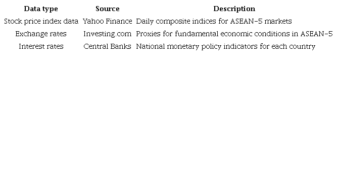
Note. Developed by the authors.

Volatility modeling analysis

The generalized autoregressive conditional heteroskedasticity (GARCH) model, effective in capturing time-varying volatility and clustering effects typically seen in financial markets, is employed to examine stock market volatility in ASEAN-5. GARCH, initially introduced by Bollerslev (1986) as an extension of Engle’s (1982) ARCH model, utilizes historical returns and volatility to deliver a more precise estimation of volatility patterns. This is ideal for examining volatility spillovers, as it demonstrates the impact of volatility in one period on subsequent periods - an essential factor in the analysis of interconnected markets like those of ASEAN-5. Prior studies, such as those conducted by Boonyakunakorn et al. (2019) and Darinda and Permana (2019), validate the effectiveness of GARCH in analyzing risk and spillover effects in developing nations.

The study employs lagged variables and control variables within the GARCH model to address endogeneity, which may arise from reciprocal linkages between markets. Lag structures reduce bias by delineating the direction of volatility transmission, thereby preventing simultaneous feedback effects. Additionally, winsorization was applied to adjust extreme values to the 1st and 99th percentiles, thereby addressing outliers that frequently result from atypical market movements. This method mitigates the impact of outliers while preserving the dataset’s integrity and variability, thus providing a more accurate representation of typical market behavior untainted by rare occurrences.

The first step in modeling GARCH is to build the autoregressive (AR) model, which is a type of model in time series analysis and used to understand and predict future values based on past values from a time series (Tsay, 2005). In the AR(p) model, p indicates the number of lags or delays used in the model. That is, the current value is predicted based on the previous p value. Therefore, AR(p) modeling can be used to model the average of a time series, with the AR(p) equation as follows.

Where y_tx is the return of each joint stock from each country at time t; β is a constant value; and θ_i is the regression coefficient AR(p) with i = 1,2,3, ...., p.

Next, to build a robust model, we test for heteroscedasticity by modeling volatility using ARCH (Engle, 1982). Tsay (2014) states that this model relates the conditional variance of disturbances to a linear combination of past squared disturbances. To ensure the existence of an ARCH effect, the best ARMA model selected must be checked using the Lagrange multiplier (LM) test (Nelson, 1991).

The next step is to model GARCH, introduced by Bollerslev (1986). The GARCH model is used to avoid high-order ARCH models and can be applied to observe several residual relationships that also depend on several previous residuals. Since the conditional variance is related to the conditional variance of the previous lag allowed in the GARCH model, the equation is presented as follows:

Where σ_t² is the conditional variance at time t, α₀ is the intercept, ε_t²_-j is the residual from the previous period, σ_t²_{- k} is the conditional variance from the previous period, φ_j is the ARCH coefficient, and δ_k is the GARCH coefficient.

Chuang and Wei (1991) stated that the heteroscedasticity of the conditional variance varying over time from the GARCH model exists in AR and MA, where the lag q of the squared residual and the lag p of the conditional variance are denoted as GARCH(p,q).

Modeling analysis of relationships between capital markets

In this work, the modeling of linkages between capital markets will apply the vector autoregressive (VAR) model or the vector error correction model (VECM). The VAR model is a statistical method used to handle and predict dynamic systems with several interrelated variables (Hamzah et al., 2020). Each variable in the VAR model is treated as a linear function of its own previous values and those of other variables in the system. However, the traditional VAR model is insufficient when the given data exhibit co-integration characteristics, namely the existence of a stable long-term relationship between these variables (Hair et al., 2014). To overcome this problem, the VECM model is used, which incorporates error correction mechanisms into the model, thereby enabling a closer examination of long- and short-term correlations between variables (Singh & Joshi, 2019).

To ensure the validity and robustness of the VAR and VECM models, the following tests and validation methods were conducted: stationarity testing via the augmented Dickey-Fuller (ADF) Test, co-integration testing using the Johansen co-integration test, optimal lag length determination using lag selection criteria such as AIC, SC, and HQ, impulse response function (IRF), and variance decomposition.

Investment risk analysis (VaR assessment)

VaR is a methodology used to analyze maximum loss data in investment decisions (Tsay, 2005). This study employs the variance-covariance approach due to its computational efficiency and seamless integration with volatility estimates derived from the AR(p)-GARCH(p,q) model. VaR was calculated at 95% and 99% confidence levels over a 15-day horizon using daily return data from ASEAN-5 markets. The formula for calculating VaR using the variance-covariance approach is as follows (Tsay, 2005):

Where μ: mean; σ: volatility; α: confidence level; t: time period.

VaR was chosen for its simplicity, widespread acceptance, and ability to provide a clear measure of potential losses (Tsay, 2005). Compared to other methods, historical simulation captures real market behavior but relies heavily on past data trends (Hull, 2015). Meanwhile, Monte Carlo simulation offers flexibility at the expense of increased computational demands (Alexander, 2008). Conditional VaR (CVaR) and expected shortfall (ES) provide more comprehensive assessments of tail risk, addressing VaR’s limitation of neglecting extreme losses beyond the threshold (Acharya et al., 2011). Despite its practicality, VaR has limitations, including its assumption of normal return distributions and potential underestimation of extreme risks - factors particularly relevant in the volatile ASEAN-5 markets.

RESULTS AND DISCUSSION

Stationary data tests

The following are graphs plotting the combined share prices of each ASEAN-5 countries for 2019-2023.

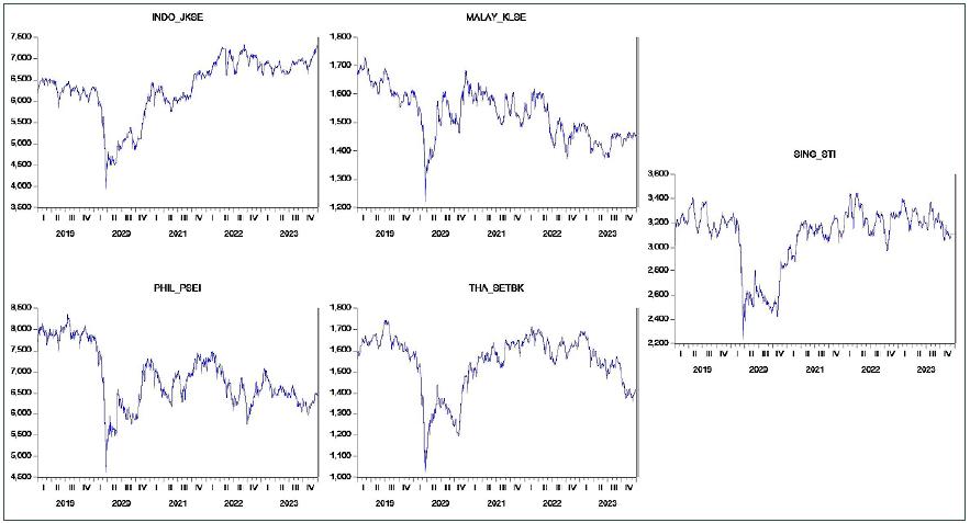
Figure 1
Plotting stock index prices in each ASEAN-5 country 2019-2023
Source: Yahoo Finance (2024).World Indices. https://finance.yahoo.com/markets/world-indices/

Over the last five years, the ASEAN-5 stock markets have exhibited notable patterns. The Jakarta composite index (JKSE) was stable around 6,500 points at the beginning of 2019 with minor fluctuations. However, it fell sharply to 3,500 points in early 2020 due to the COVID-19 pandemic. JKSE recovered significantly between 2020 and 2021, consolidated with swings near 7,000 points in 2022, and rose past 7,000 points in 2023. Similarly, the Malaysia Bursa index (KLSE) showed a declining trend around 1,700 points in 2019, dropped to 1,200 points in 2020 due to the pandemic, recovered to 1,600 points by the end of 2021, and displayed fluctuations around 1,400 points throughout 2022, remaining stable between 1,400 and 1,450 points until mid-2023. The Philippines stock exchange index (PSEI) started at around 8,000 points in 2019, then dropped sharply to almost 4,500 points in 2020 due to the pandemic. It recovered to nearly 7,000 points by the end of 2021 but showed a declining trend with oscillations between 6,000 and 7,000 points in 2022, stabilizing around 6,000 to 6,500 points by mid-2023. The stock exchange of Thailand (SET) index, which was around 1,600 to 1,700 points in early 2019, experienced a significant drop to nearly 1,000 points in 2020 due to the pandemic. It gradually recovered in 2020 and 2021, consolidated around 1,600 and 1,700 points in 2022, and showed stability with variations between 1,600 to 1,800 points in 2023. Lastly, the Singapore straits times index (STI) began 2019 around 3,200 to 3,300 points, fell to 2,200 points in 2020 due to COVID-19, and recovered to nearly 3,200 points by the end of 2021. The STI exhibited a steady trend with fluctuations between 3,000 and 3,200 points throughout 2022, maintaining this range until the end of 2023.

A further stage is to run the stationarity test to ensure that the data used in the GARCH model analysis is stationary. The stationarity test results using the augmented Dickey-Fuller (ADF) test are presented in Table 2.

Table 2

ADF test results (level).

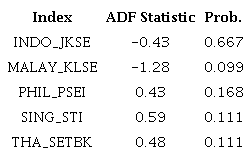
Note. Processed data (2024).

From the ADF test results in Table 2, all composite stock price indices have a probability value greater than 0.05, indicating that the data has a unit root and is not stationary at level. Therefore, differencing is carried out at the first level (d = 1) to make the data stationary. The ADF test results after differencing are presented in Table 3.

Table 3

ADF test results (differencing 1).

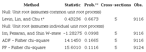
Note. ** Probabilities for Fisher tests are computed using an asymptotic chi-square distribution. All other tests assume asymptotic normality. Processed data (2024).

After differencing, all stock price indices show a very significant probability (less than 0.05), which means the data has become stationary and is ready to be analyzed using the AR(p)-GARCH(p,q) model.

Volatility analysis

The ADF unit root test results at differencing level 1 (d = 1), in Table 3, show that the data series’ volatility is stable. Homoscedasticity - that is, constant variance - is a fundamental assumption behind ordinary least squares (OLS) regression. OLS loses efficiency if the variation is heteroscedastic - that is, not constant. One should apply the AR(p)-GARCH(p,q) model, which considers heteroscedasticity, to solve this. The ARCH effect test helps identify heteroscedasticity prior to applying the AR(p)-GARCH(p,q) model. With values smaller than 0.05, the Q and LM portmanteau tests verify the existence of ARCH effects in the volatility variances of the ASEAN-5 composite stock index. Accurate mean and volatility estimations depend on AR(p)-GARCH(p,q). The results of the model for each composite stock index are attached in Appendix 2 (https://data.mendeley.com/datasets/sct6z9jsf6/1).

The parameter estimates of the GARCH model for Indo_JKSE are statistically significant. AR(1) coefficient estimation is close to -1, indicating a very strong negative autoregression. The significant ARCH(1) and GARCH(1) coefficients indicate that current volatility is strongly influenced by the squared residuals from the previous period and the previous variance. Therefore, it can be concluded that the AR(p)-GARCH(p,q) model for the stock price index in Indonesia (Indo_JKSE) is AR(1) - GARCH(1,1), with the model estimation as follows:

Next, parameter estimation for Malay_KLSE shows that the AR(1) parameter, which is close to -1, indicates strong negative autoregression. The significant ARCH(1) and GARCH(1) coefficients indicate that current volatility is influenced by the square of the residual and previous variance. Therefore, it can be concluded that the AR(p)-GARCH(p,q) model for the stock price index in Malaysia (Malay_KLSE) is AR(1) - GARCH(1,1), with the model estimation as follows:

Volatility in the Philippine stock market is influenced by the squared residuals of the two previous periods (ARCH(1) and ARCH(2)), as well as the variance of the two previous periods (GARCH(1) and GARCH(2)). So, the AR(p)-GARCH(p,q) model for the stock price index in the Philippines (Phil_PSEI) is AR(1) - GARCH(2,2), with the model estimation as follows:

Volatility estimation in the Singapore stock market is influenced by the squared residual from the previous period (ARCH(1)) and the previous variance (GARCH(1)). The AR(1) coefficient shows a very strong negative autoregression. So, the AR(p)-GARCH(p,q) model for the stock price index in Singapore (Sing_STI) is AR(1) - GARCH(1,1), with the model estimation as follows:

Finally, the Thai stock market is influenced by the squared residual from the previous period (ARCH(1)) and the previous variance (GARCH(1)). The AR(1) coefficient shows a very strong negative autoregression. Therefore, it can be concluded that the AR(p)-GARCH(p,q) model for the stock price index in Thailand (Thai_SETBK) is AR(1) - GARCH(1,1), with the model estimation as follows:

The study of the stock markets in Indonesia (Indo_JKSE), Malaysia (Malay_KLSE), the Philippines (Phil_PSEI), Singapore (Sing_STI), and Thailand (Thai_SETBK) reveals notable volatility in every market. Indicating continuous volatility across all markets, the GARCH model shows that both the ARCH component (squared residual) and the GARCH component (prior variance) significantly affect present volatility. A high GARCH coefficient in Indonesia indicates long-lasting consequences of volatility shocks, reflecting constant high volatility. Malaysia’s market similarly exhibits notable - though somewhat less pronounced - volatility persistence. Though less erratic than Indonesia and Malaysia, the market in the Philippines also displays significant GARCH characteristics. With a relatively high GARCH value suggesting long-lasting volatility effects, Singapore’s market exhibits pronounced volatility. With a GARCH coefficient close to 1, Thailand’s market shows strong volatility with clear persistence. For risk managers and investors, high volatility offers both greater risk and profit potential. Investors should consider the volatility of their strategies and use diversification to reduce risk. Employing strict risk mitigation tactics and derivative instruments, risk managers must take volatility persistence into account when setting risk limits and creating hedging strategies. GARCH modeling demonstrates that foreign market shocks significantly affect the volatility of Southeast Asian financial markets, thus offering valuable new insights. Policymakers and investors seeking to make informed decisions and manage market volatility effectively must take this understanding into account.

Analysis of the relationship between the ASEAN-5 composite stock index - volatility spillover

Given the framework of interconnected global financial markets, shocks in one market might affect volatility in another. Lamine et al. (2024) emphasized the importance of market interconnection in global volatility by showing how volatility in one market can influence others. For example, variations in the stock markets of Singapore or Thailand can affect changes in other regional stock markets, such as those of Malaysia and Indonesia. Although GARCH modeling reveals that, to some extent, volatility in these markets is relatively structured and predictable, external factors still need to be considered. Therefore, further knowledge of the interactions among the ASEAN-5 markets should be obtained through additional studies, including the estimation of causal models.

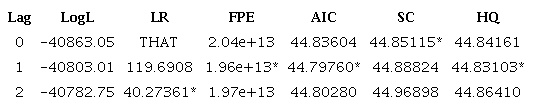
From Table 3, we observe that the composite stock price index data series in each ASEAN-5 country has become stationary at the first differencing level (d = 1). VAR and VECM models require a stationary dataset for analysis. Before estimating the parameters of the causal relationship model, the dataset is first tested by determining the optimal lag to more accurately explain the dynamic model. Table 4 presents the estimated parameters for determining the optimal lag from the combined stock price dataset in the ASEAN-5 countries.

Table 4

Estimation parameter of schematic representation (lag optimal).

Note. * Indicates lag order selected by the criterion.

Table 4 shows the results of optimal lag selection with endogenous variables D(JKSE), D(KLSE), D(PSEI), D(STI), and D(SETBK), as well as the exogenous variable C, with a total of 1,823 observations. Several selection criteria used are LogL (log likelihood), LR (sequential modified LR test statistic), FPE (final prediction error), AIC (Akaike information criterion), SC (Schwarz information criterion), and HQ (Hannan-Quinn information criterion). Based on Table 4, we see that the AIC and FPE criteria select lag 1 as the optimal lag, with AIC and FPE values of 44.79760 and 1.96e+13, respectively - the lowest among all lags. The HQ criterion also indicates lag 1 with a value of 44.83103. However, the SC criterion shows the optimal lag at lag 0, with a value of 44.85115. Overall, most selection criteria (AIC, FPE, and HQ) choose lag 1 as the optimal lag in modeling the dynamic relationships between variables. Thus, lag 1 can be considered the most appropriate lag to use in this model to estimate the relationships between the stock market variables studied.

Cointegration test

After obtaining the optimal lag in estimating model parameters, the next step is to carry out a cointegration test to determine which model is appropriate to use, whether the VAR or VECM model. The trace test results in the Johansen cointegration test (Appendix 2 https://data.mendeley.com/datasets/sct6z9jsf6/1) show that there are five cointegration equations that are significant at the 5% level. This is proven by the trace statistic which is greater than the critical value at each hypothesis level. For example, the null hypothesis ‘none,’ with an eigenvalue of 0.386676, yields a trace statistic of 3990.159, well above the critical value of 69.81889, with a probability of 1.0000. Likewise, the hypotheses ‘at most 1’ and ‘at most 2’ show trace statistics of 3098.965 and 2228.044 respectively, which also exceed the relevant critical value. The maximum eigenvalue test results also show that there are five cointegration equations that are significant at the 5% level. The null hypothesis ‘none,’ with an eigenvalue of 0.386676, yields a statistic of 891.1943, well above the critical value of 33.87687, with a probability of 0.0001. The hypotheses ‘at most 1’ and ‘at most 2’ show statistics of 870.9213 and 815.0262, respectively, which are also higher than the relevant critical values. The normalized cointegration coefficient, as well as the adjustment coefficient, shows the various relationships and influences between these variables, as well as how each variable adjusts to maintain the long-term relationship.

Based on the results of the Johansen cointegration test, which show a significant cointegration relationship among the variables tested, the most appropriate model to use is the VECM. This is because VECM can incorporate the long-run relationships found among these variables, allowing for an error adjustment component that shows how quickly the variables return to long-term equilibrium after deviations, as well as allowing analysis of long- and short-term relationships. Therefore, VECM modeling can be further analyzed to provide a more comprehensive picture of the long- and short-term dynamics of the stock market variables being analyzed.

VECM model cointegration modeling

To examine the long-term equilibrium and short-term dynamics among the ASEAN-5 stock markets, this study employs the vector error correction model (VECM). The VECM is appropriate when variables are non-stationary at level but co-integrated, indicating the presence of a stable long-term relationship despite short-term fluctuations. This model allows for simultaneous analysis of both short-term adjustments and long-term equilibrium corrections, providing insight into how shocks in one market affect others over time.

The cointegration analysis was conducted using the Johansen test to identify the existence and number of cointegrating vectors among the five stock indices. Once cointegration was confirmed, the VECM(1) model was estimated, incorporating one lag based on the optimal lag selection criteria. The error correction term (ECT) in the model reflects the speed of adjustment toward the long-term equilibrium after a shock, while the differenced variables capture short-term interactions. The output for the vector error correction estimates is attached in Appendix 3 (https://data.mendeley.com/datasets/sct6z9jsf6/1)

The following is the VECM(1) model equation based on Appendix 3 (https://data.mendeley.com/datasets/sct6z9jsf6/1), which includes the cointegration equation and the error correction equation.

In the cointegration equation (Equation 14), D(JKSE) is the dependent variable. Positive coefficients for D(KLSE) (0.2819) and D(PSEI) (0.1283) indicate a positive long-term relationship with D(JKSE), while negative coefficients for D(STI) (-1.3456) and D(SETBK) (-2.1568) suggest an inverse relationship. The constant term is -0.6174. In the error correction model (Equations 15-19), the coefficient of CointEq1 for D(JKSE,2) (-0.7099) shows a quick adjustment back to equilibrium after deviations, with D(JKSE(-1),2) having a significant negative effect (-0.1159) and D(PSEI(-1),2) a positive effect (0.2181). D(STI(-1),2) and D(SETBK(-1),2) negatively impact D(JKSE,2).

This VECM model also shows several model performance indicators. The R-squared value shows that about 37.7% of the variability of D(JKSE,2) can be explained by the model. A high and significant F-statistic value indicates that the overall model is significant. The log-likelihood of this model is -42332.23, with an Akaike information criterion (AIC) of 46.48627 and a Schwarz criterion (SC) of 46.60713. Overall, the VECM(1) model shows that there is a significant long-run relationship between these variables, and there is a significant adjustment to the long-run balance after deviations. This shows that the VECM model is an appropriate tool for analyzing long- and short-term dynamics between the analyzed stock market indices.

Granger causality test

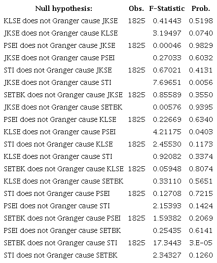
Table 5 shows the test results of pairwise Granger causality with lag 1 for variables D(JKSE), D(KLSE), D(PSEI), D(STI), and D(SETBK). This test seeks to ascertain whether one variable might be used to forecast another. The Granger causality test reveals several notable causative linkages between the investigated stock market indexes - in particular, JKSE causes changes in STI, KLSE causes changes in PSEI, and SETBK causes changes in STI. These findings confirm the application of previously estimated VECM models to describe the dynamics of long-term relationships and transient changes between several variables.

Table 5

Pairwise Granger causality tests.

Note. Processed data (2024).

Impulse response function (IRF)

Figure 2 displays the IRF applied to investigate, over time, how a shock on one variable influences another variable in the system. Responses of the variables D(JKSE), D(KLSE), D(PSEI), D(STI), and D(SETBK) to shocks in other variables are shown in the IRF graph from the VECM model with lag 1.

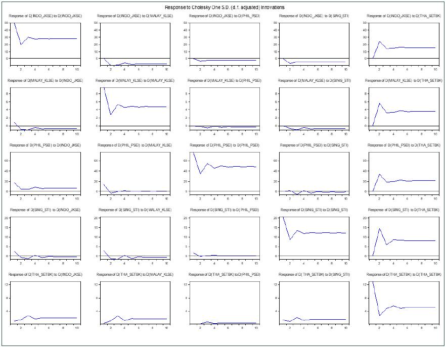
Figure 2
Impulse response function (IRF) graph for the model VECM(1).
Source: Eviews 12, Processed Data (2024).

D(JKSE) responds differently to shocks from outside markets. Shocks from D(PSEI) and D(KLSE) have little and fast-stabilizing impact on D(JKSE). Before D(JKSE) stabilizes, a shock from D(STI) clearly has a short-term negative impact. Furthermore, D(SETBK) has little effect on D(JKSE). With negligible influence from D(PSEI), D(STI), and D(SETBK), D(KLSE) shows a moderate, rapidly stabilizing negative reaction to shocks from D(JKSE). D(JKSE) shocks cause a temporary negative impact on D(PSEI); yet, with no effect from D(KLSE), D(STI), or D(SETBK) shocks, it stabilizes over time. While shocks from D(KLSE) and D(PSEI) have little impact, D(STI) exhibits a considerable initial dip due to D(JKSE) shocks and a clear drop from D(SETBK) shocks before stabilizing. D(SETBK) reacts badly to D(JKSE) shocks but promptly finds stability. While shocks from D(STI) induce a notable initial drop before stabilizing, shocks from D(KLSE) and D(PSEI) have lesser impact. The impulse response function analysis generally shows that shocks in D(STI) greatly affect D(JKSE) and D(SETBK), and that shocks in D(JKSE) clearly impact D(STI) and D(PSEI). Many more responses indicate that not all variables greatly influence one another, showing small effects and a fast return to stability

Forecast error variance decomposition (FEVD)

FEVD in the VECM model with lag 1 is used to determine the proportion of variability in a particular variable that can be explained by shocks in other variables in the system. The graphs displayed provide insight into how much each variable is affected by shocks from other variables.

Figure 3 presents the findings of the analysis demonstrating that, with quite little input from other variables, the shock itself essentially explains the variability of D(JKSE). While the contributions from D(STI) and D(SETBK) are also modest but somewhat more than those of D(KLSE), the shocks from D(KLSE) and D(PSEI) have very minor effects on the variability of D(JKSE). For D(KLSE), the shock to itself mostly explains the fluctuation. Surprises from other variables including D(JKSE), D(PSEI), D(STI), and D(SETBK) have a very modest effect on D(KLSE) variability. D(PSEI) follows the same trend; the shock itself explains most of the variability, with little help from other factors. Shocks also help to mostly explain the fluctuations in D(STI). The contribution of the shocks D(JKSE), D(KLSE), D(PSEI), and D(SETBK) to the variability of D(STI) is somewhat minor. Likewise, shocks in itself mostly explain the variability of D(SETBK); shocks from other variables including D(JKSE), D(KLSE), D(PSEI), and D(STI) play relatively minor roles in the variability of D(SETBK).

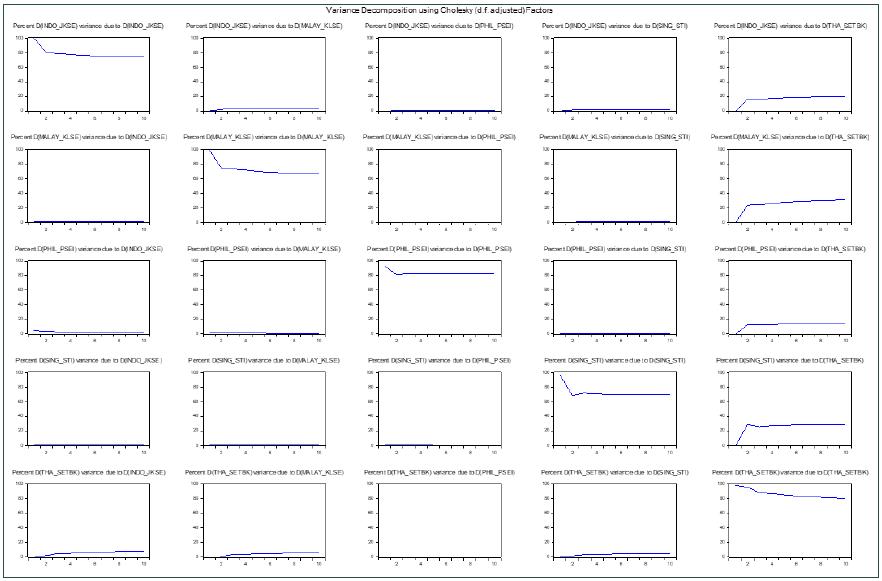
Figure 3
Forecast error variance decomposition (FEVD) graph for the model VECM(1).
Source: Eviews 12, Processed Data (2024).

The FEVD analysis reveals, in general, that shocks to the variable itself, rather than shocks from other variables in the system, explain most of the variability in each variable. This suggests that the internal dynamics of each stock market index usually have more influence than those of other stock market indices. Other variables do contribute; however, their impact is rather minor. These results are compatible with the VECM model, in which short-term effects of other variables are usually negligible, but long-term correlations between variables tend to predominate.

Investment risk level analysis (VaR assessment)

VaR is used to estimate the maximum potential loss that may occur over a certain period with a certain level of confidence. Equations (4) to (13) are AR(p)-GARCH(p,q) model equations that describe the average value and volatility of the composite stock index price for each ASEAN-5 country. These equations then become the basis for calculating the VaR value, which is used to assess the risk of investment loss in a particular portfolio. Using the average value and volatility estimated by the AR(p)-GARCH(p,q) model, we calculate the daily return distribution and then estimate the VaR, as well as daily volatility, and use them to calculate VaR at the 95% and 99% confidence levels for the following 15 days.

VaR for JKSE

To calculate the VaR for the Indo_JKSE index, the parameter estimation results from the AR(1)-GARCH(1,1) model are used as in Equations (4) and (5). From Appendix 1 (https://data.mendeley.com/datasets/sct6z9jsf6/1), it is known that the total observation data is 1826, so the JKSEt-1 value is 7273; ε_t²_-1 is -1932.25; and σ_t²_-1 is 9205.25. Then, the data above is substituted into Equations (4) and (5) as attached in Appendix 4. https://data.mendeley.com/datasets/sct6z9jsf6/1

VaR for KLSE

To calculate the VaR on the Malay_KLSE index, the estimation results in Equations (6) and (7), namely the AR(1)-GARCH(1,1) model, are used. From Appendix 1 (https://data.mendeley.com/datasets/sct6z9jsf6/1), it is known that the total observation data is 1826, so the KLSEt-1 value is 1455; ε_t²_-1 is 2.01; and σ_t²_-1 is 7410.73. Then, the data above is substituted into Equations (6) and (7) as attached in Appendix 4 (https://data.mendeley.com/datasets/sct6z9jsf6/1).

VaR for PSEI

To calculate the VaR on the Phil_PSEI index, the estimation results in Equations (8) and (9), namely the AR(1)-GARCH(2,2) model, are used. From Appendix 1 (https://data.mendeley.com/datasets/sct6z9jsf6/1), it is known that the total observation data is 1826, so the PSEIt-1 value is 6450; ε_t²_-1 is 0.00006; and σ_t²_-1 is -0.000056508. Then, the data above is substituted into Equations (8) and (9) as attached in Appendix 4 (https://data.mendeley.com/datasets/sct6z9jsf6/1)

VaR for STI

To calculate the VaR on the Sing_STI index, the estimation results in Equations (10) and (11), namely the AR(1)-GARCH(1,1) model, are used. From Appendix 1 (https://data.mendeley.com/datasets/sct6z9jsf6/1), it is known that the total observation data is 1826, so the STIt-1 value is 3111; ε_t²_-1 is 0.068; and σ_t²_-1 is 3110.93. Then, the data above is substituted into Equations (10) and (11) as attached in Appendix 4 (https://data.mendeley.com/datasets/sct6z9jsf6/1).

VaR for SETBK

To calculate the VaR on the Thai_SETBK index, the estimation results in Equations (12) and (13), namely the AR(1)-GARCH(1,1) model, are used. From Appendix 1 (https://data.mendeley.com/datasets/sct6z9jsf6/1), it is known that the total observation data is 1826, so the SETBKt-1 value is 1416; ε_t²_-1 is 3.09; and σ_t²_-1 is 17475.94. Then the data above is substituted into Equations (12) and (13) as attached in Appendix 4 (https://data.mendeley.com/datasets/sct6z9jsf6/1).

VaR measurement is an important tool in investment risk management, used to measure the maximum potential loss in a portfolio within a certain period and at a given level of confidence. The results of VaR calculations for various composite stock indices in several countries provide an overview of the potential risks that investors may face in their respective markets. Based on the applied AR(1)-GARCH(1,1) model, VaR calculations were carried out for the composite stock price index of Indonesia (JKSE), Malaysia (KLSE), the Philippines (PSEI), Singapore (STI), and Thailand (SETBK).

VaR at the 95% confidence level for JKSE is approximately 967.16. This suggests that, during the next 15 days, the maximum loss will not surpass 967.16 with a 95% likelihood. Reflecting the danger of a notable price drop, the average value of JKSE at time t, computed using the AR(1) model, indicates a negative value. With a daily volatility computed using the GARCH(1,1) model of 586.16, the Indonesian stock market exhibits a significant degree of volatility. High volatility and the possibility of significant maximum losses in an investment environment point to the extreme risk this market presents but also indicate great profit possibilities for investors who can properly manage risk (Shrydeh et al., 2019).

Under a 95% confidence level, the VaR for KLSE is roughly 352.91. With the AR(1) model, KLSE’s average value at time t is 213.87, suggesting a more consistent rise in expectations than in JKSE. With a daily volatility computed using the GARCH(1,1) model of 84.26, which is rather lower than the JKSE, the Malaysian stock market shows a more under control risk level. Though their returns should be more consistent, investors still have to be vigilant about the hazards associated (Bouri et al., 2017).

Under a 95% confidence level, the VaR for PSEI is around 821.74. Using the AR(1) model, the average PSEI value at time t is 821.73, suggesting a more consistent rise in expectations than in JKSE. With a daily volatility computed using the GARCH(1,1) model of 84.26, which is rather lower than that of JKSE, the Malaysian stock market shows a more controlled risk level. Though returns should be more consistent, investors still have to be vigilant about the associated risks (Danila, 2023).

The VaR at the 95% confidence level for STI is about 23.7. With a predicted decline, the average STI value at time t using the AR(1) model is -62.78. With a daily volatility computed using the GARCH(1,1) model of 52.4, the degree of risk is somewhat moderate. Still, the low VaR value shows that, in this market, the risk of loss is more controlled than in the other markets examined, thus it can be a wise choice for investors seeking stability (Jebabli et al., 2022).

At the 95% confidence level, the VaR for SETBK is approximately 363.83. Using the AR(1) model, the average SETBK value at time t is 153.25, suggesting a consistent rise in expectations. With a daily volatility measured using the GARCH(1,1) model of 127.62, there is clearly high volatility. Although this market offers great profit prospects, it also carries significant risk (Diebold & Yilmaz, 2009).

The outcomes of this VaR computation provide a general picture of the possible risks and returns in different stock markets. Investors must consider the degree of volatility and maximum probable loss potential and adopt suitable risk management techniques, including portfolio diversification and the use of derivative instruments for hedging. Making wiser and more strategic investment decisions, as well as properly managing risk in dynamic financial markets, depends on investors and portfolio managers understanding VaR.

Analysis volatility spillover and investment risk level

The selected study period (2019-2023) was chosen to analyze the effects of the COVID-19 pandemic, which caused significant volatility in global financial markets, including those of the ASEAN-5. The pandemic-induced economic disruptions led to frequent price fluctuations, shifts in investor sentiment, and heightened risk aversion, all of which significantly impacted stock markets. Consistent with Engle and Bollerslev (1986), the AR-GARCH model results demonstrate that past volatility substantially influences current market volatility. High GARCH coefficients in the JKSE and KLSE indicate prolonged volatility shocks, aligning with Darinda and Permana (2019), who observed similar volatility persistence in ASEAN-5 markets driven by oil price fluctuations. Danila (2023) reported strong bidirectional volatility spillovers between ASEAN and GCC markets; however, this study reveals asymmetric spillovers within the ASEAN-5, with Singapore’s STI acting as a volatility transmitter and Indonesia’s JKSE as the primary receiver. This asymmetry may stem from differences in market size, economic structure, liquidity, and investor behavior. Singapore’s global financial integration allows external shocks to quickly permeate regional markets, whereas Indonesia’s dependence on commodity exports and higher retail investor participation may amplify volatility persistence.

Further exploration of volatility asymmetry reveals institutional and behavioral factors contributing to Indonesia’s higher volatility persistence. Indonesia’s financial markets, with substantial retail investor activity, often experience herd behavior and overreactions to news, exacerbating volatility shocks (Mensi et al., 2021). Institutional inefficiencies, such as delayed regulatory responses and lower market liquidity, also prolong volatility. Conversely, Singapore’s mature regulatory environment and diversified economy mitigate prolonged volatility, underscoring its role as a regional stabilizer. Malaysia’s KLSE, with moderate volatility persistence, benefits from balanced foreign and local investor participation and a stable macroeconomic framework, which tempers volatility spillovers despite external shocks.

The value at risk (VaR) calculations, based on the AR(p)-GARCH(1,1) model, highlight significant differences in market risk profiles. At a 95% confidence level over a 15-day horizon, the JKSE’s VaR of 967.16 indicates Indonesia’s heightened risk exposure, reflecting its economic reliance on volatile sectors and sensitivity to both global and local shocks. This finding supports Boonyakunakorn et al. (2019), who identified Indonesia as having a higher risk profile within ASEAN markets. In contrast, the KLSE and PSEI exhibit lower VaR values, signaling reduced risk exposure. Singapore’s STI maintains controlled volatility with lower VaR, consistent with its diversified economic base and mature financial systems.

The VECM analysis reveals a long-term equilibrium relationship among ASEAN-5 stock indices, indicating that volatility spillovers from COVID-19-related shocks were not confined to individual markets. The cointegration equation shows that fluctuations in the STI and SETBK significantly affect the JKSE, aligning with Diebold and Yilmaz (2009), who emphasized the global nature of volatility spillovers. The findings demonstrate that systemic risk in ASEAN-5 markets is heightened during global crises, with volatility shocks propagating through interconnected financial systems. Notably, external factors such as geopolitical tensions (e.g., South China Sea disputes) and global trade disruptions further intensify regional market volatility, highlighting the vulnerability of ASEAN-5 markets to external shocks.

Comparing this study with existing literature reveals both consistencies and divergences. Unlike Bautista and Mora (2021), who noted the resilience of some ASEAN markets, this study underscores limited diversification benefits within the ASEAN-5 due to strong market interconnections. Our results suggest that Indonesia and Thailand remain highly susceptible to regional volatility, diminishing cross-market diversification effectiveness, while Bautista and Mora (2021) found that certain markets like Malaysia and Singapore provided buffers during regional disruptions. Lamine et al. (2024) similarly argued that systemic shocks within ASEAN markets often undermine diversification strategies. Additionally, the asymmetry in volatility transmission observed in this study contrasts with findings from Danila (2023), where bidirectional spillovers were more prominent in ASEAN-GCC relations, suggesting regional variations in market interconnectedness.

Exploring the causes of volatility transmission asymmetry, economic structure differences play a pivotal role. Singapore’s STI, as a global financial hub with significant foreign investment and robust regulatory frameworks, efficiently transmits external shocks but absorbs them quickly. Conversely, Indonesia’s JKSE, reliant on commodity exports and characterized by less market depth, experiences prolonged volatility as local market participants react more strongly to global developments. Behavioral factors, including higher retail investor participation in Indonesia and Thailand, contribute to overreactions to market news, exacerbating volatility shocks. Institutional factors, such as regulatory lag and political uncertainty in Thailand, further intensify volatility persistence.

The comparative analysis highlights clear volatility spillover patterns: Singapore and Thailand serve as volatility transmitters, significantly influencing neighboring markets, particularly Indonesia and Malaysia. Conversely, Indonesia and the Philippines act as volatility receivers, with weaker reciprocal effects. This interdependence underscores the challenges ASEAN-5 investors face when seeking effective cross-market diversification, as systemic shocks tend to propagate regionally, limiting potential risk mitigation.

VaR analysis further confirms Indonesia’s elevated risk profile, followed by Thailand and the Philippines, while Malaysia and Singapore exhibit lower risk levels. These divergences underscore the necessity for tailored risk management strategies. Markets prone to prolonged volatility, like Indonesia and Thailand, require enhanced hedging mechanisms and diversified investments in less volatile regions. Policymakers should consider structural reforms to improve market resilience, enhance regulatory responsiveness, and reduce investor overreaction.

All in all, this study’s findings emphasize the importance of incorporating volatility spillover effects into investment strategies within the ASEAN-5. The significant interdependence among markets suggests that regional diversification alone may not sufficiently mitigate systemic risk. Investors should adopt comprehensive risk mitigation strategies, such as using derivatives for hedging and diversifying into global markets with lower volatility and reduced interconnection (Jebabli et al., 2022). Portfolio managers must understand these volatility dynamics to optimize returns and manage risks in an increasingly interconnected financial environment.

CONCLUSION

This research offers significant insights into the dynamics of volatility and investment risk within ASEAN-5 markets, highlighting robust interconnections and systemic risk, especially in relation to the COVID-19 pandemic. Employing AR-GARCH and VECM models, our analysis indicates that volatility exhibits persistence and is significantly affected by historical values, with market shocks propagating to others, thereby highlighting the interconnectedness of the ASEAN-5 markets. The value at risk (VaR) analysis demonstrates that the Indonesian stock market (JKSE) exhibits a higher risk profile relative to other ASEAN-5 markets, highlighting the diverse levels of risk exposure across the region. The findings indicate that investors ought to exercise caution regarding cross-market diversification within the ASEAN-5, as it may not adequately reduce systemic risk. Furthermore, it is advisable to implement supplementary risk management strategies, including hedging or diversifying into markets with lower volatility.

The selected analysis period (2019-2023) encompasses the pre-pandemic, pandemic, and recovery phases, with the objective of evaluating the pandemic’s substantial influence on volatility in ASEAN-5 markets. The COVID-19 pandemic induced significant market volatility, swift changes in investor sentiment, and heightened risk aversion, factors that persist in influencing the financial landscape. Moreover, external factors like political crises and geopolitical tensions, including trade disputes and regional conflicts, add complexity by increasing uncertainty and volatility in ASEAN-5 markets. These factors influence investor confidence and market stability, exacerbating the systemic risks inherent in these interconnected markets.

This study addresses a significant gap in the literature by integrating volatility spillover analysis with VaR-based risk assessment in the context of the ASEAN-5 during a transformative period. The findings have practical implications for both investors and policymakers. Investors should implement risk mitigation strategies like derivative hedging and diversify beyond the ASEAN-5 markets to reduce systemic risk. Policymakers are encouraged to enhance regional cooperation, establish early warning systems, and promote regulatory transparency to improve market stability.

However, the study has limitations, including the use of aggregate data that may overlook sector-specific effects, and the focus on stock market indices without considering other financial instruments. The models applied primarily capture linear relationships, potentially missing non-linear market dynamics. Future research could address these gaps by examining sector-specific volatility, exploring longer economic cycles, and incorporating non-linear models to better understand market behavior. Additionally, studying the impact of specific macroeconomic indicators and institutional factors could provide a more nuanced view of volatility spillovers and investment risks in emerging markets.

REFERENCES

Acharya, V. V., Brownlees, C., Engle, R., Farazmand, F., & Richardson, M. (2011). Measuring Systemic Risk. Regulating Wall Street: The Dodd-Frank Act and the New Architecture of Global Finance, May, 85-119. https://doi.org/10.1002/9781118258231.ch4

Acharya, V. V., Pedersen, L. H., Philippon, T., & Richardson, M. (2017). Measuring systemic risk. Review of Financial Studies, 30(1), 2-47. https://doi.org/10.1093/rfs/hhw088

Adekoya, O. B., & Oliyide, J. A. (2021). How COVID-19 drives connectedness among commodity and financial markets: Evidence from TVP-VAR and causality-in-quantiles techniques. Resources Policy, 70(October 2020), 101898. https://doi.org/10.1016/j.resourpol.2020.101898

Ahadiat, A., & Kesumah, F. S. D. (2021). Risk Measurement and Stock Prices during the COVID-19 Pandemic: An Empirical Study of State-Owned Banks in Indonesia*. Journal of Asian Finance, 8(6). http://dx.doi.org/10.13106/jafeb.2021.vol8.no6.0819

Alexander, C. (2008). Market Risk Analysis: Quantitative Methods in Finance. John Wiley & Sons.

Bautista, R. S., & Mora, J. A. N. (2021). Value-at-risk predictive performance: a comparison between the CaViaR and GARCH models for the MILA and ASEAN-5 stock markets. Journal of Economics, Finance and Administrative Science, 26(52), 197-221. https://doi.org/10.1108/JEFAS-03-2021-0009

Bodea, C., & Hicks, R. (2015). International Finance and Central Bank Independence: Institutional Diffusion and the Flow and Cost of Capital. The Journal of Politics, 77(1), 268-284. https://doi.org/10.1086/678987

Bollerslev, T. (1986). Generalized Autoregressive Conditional Heteroskedasticity. Journal of Econometrics, 31(1), 307-327. https://doi.org/10.1109/TNN.2007.902962

Boonyakunakorn, P., Pastpipatkul, P., & Sriboonchitta, S. (2019). Value at risk of the stock market in asean-5. In Studies in Computational Intelligence (Vol. 809). Springer International Publishing. https://doi.org/10.1007/978-3-030-04200-4_33

Bouri, E., Jain, A., Biswal, P. C., & Roubaud, D. (2017). Cointegration and nonlinear causality amongst gold, oil, and the Indian stock market: Evidence from implied volatility indices. Resources Policy, 52(February), 201-206. https://doi.org/10.1016/j.resourpol.2017.03.003

Chen, Y. H., Hsu, I. C., & Lin, C. C. (2010). Website attributes that increase consumer purchase intention: A conjoint analysis. Journal of Business Research, 63, 1007-1014. https://doi.org/10.1016/j.jbusres.2009.01.023

Chuang, A., & Wei, W. W. S. (1991). Time Series Analysis: Univariate and Multivariate Methods. In Technometrics, 33(1), 108). https://doi.org/10.2307/1269015

Danila, N. (2023). Spillover of volatility among financial instruments: ASEAN-5 and GCC market study. PLoS ONE, 18(10 October), 1-21. https://doi.org/10.1371/journal.pone.0292958

Darinda, D., & Permana, F. C. (2019). Volatility Spillover Effects In Asean-5 Stock Market: Does The Different Oil Price Era Change The Pattern? Kajian Ekonomi Dan Keuangan, 3(2), 116-134. https://doi.org/10.31685/kek.v3i2.484

Diebold, F. X., & Yilmaz, K. (2009). Measuring Financial Asset Return and Volatility Spillovers, With Application To Global Equity Markets. The Economic Journal, 119, 158-171. http://www.nber.org/papers/w13811

Engle, R. F. (1982). Autoregressive Conditional Heteroscedasticity with Estimates of the Variance of United Kingdom Inflation. Econometrica, 50(4), 987. https://doi.org/10.2307/1912773

Engle, R. F., & Bollerslev, T. (1986). Modelling the persistence of conditional variances. Econometric Reviews, 5(1), 1-50. https://doi.org/10.1080/07474938608800095

Engle, R. F., & Manganelli, S. (2004). CAViaR: Conditional autoregressive value at risk by regression quantiles. Journal of Business and Economic Statistics, 22(4), 367-381. https://doi.org/10.1198/073500104000000370

Hair, J. F., Jr., Black, W. C., Babin, B. J., & Anderson, R. E. (2014). Multivariate Data Analysis (Pearson Ne). Pearson Education Limited.

Hamzah, L. M., Nabilah, S. U., Russel, E., Usman, M., Virginia, E., & Wamiliana. (2020). Dynamic Modelling and Forecasting of Data Export of Agricultural Commodity by Vector Autoregressive Model. Journal of Southwest Jiaotong University, 55(3). https://doi.org/10.35741/issn.0258-2724.55.3.41

Horvath, R., & Petrovski, D. (2013). International stock market integration: Central and south eastern europe compared. Economic Systems, 37(1), 81-91. https://doi.org/10.1016/j.ecosys.2012.07.004

Hull, J. C. (2015). Risk Management and Financial Institutions. John Wiley & Sons.

Jebabli, I., Kouaissah, N., & Arouri, M. (2022). Volatility spillovers between stock and energy markets during crises: A comparative assessment between the 2008 Global Financial Crisis and the Covid-19 Pandemic Crisis. Finance Research Letters, 46(July), 102363. https://doi.org/10.1016/j.frl.2021.102363

Jovanović, M. N., & Lipsey, R. G. (2006). International economic integration: Limits and prospects. In International Economic Integration: Limits and Prospects. https://doi.org/10.4324/9780203019894

Lamine, A., Jeribi, A., & Fakhfakh, T. (2024). Spillovers between cryptocurrencies, gold and stock markets: implication for hedging strategies and portfolio diversification under the COVID-19 pandemic. Journal of Economics, Finance and Administrative Science, 29(57), 21-41. https://doi.org/10.1108/JEFAS-09-2021-0173

Liu, F., Umair, M., & Gao, J. (2023). Assessing oil price volatility co-movement with stock market volatility through quantile regression approach. Resources Policy, 81, 103375. https://doi.org/10.1016/J.RESOURPOL.2023.103375

Liu, Y., Wei, Y., Wang, Q., & Liu, Y. (2022). International stock market risk contagion during the COVID-19 pandemic. Finance Research Letters, 45(February 2021), 102145. https://doi.org/10.1016/j.frl.2021.102145

Mensi, W., Hammoudeh, S., Nguyen, D. K., & Kang, S. H. (2016). Global financial crisis and spillover effects among the U.S. and BRICS stock markets. International Review of Economics and Finance, 42, 257-276. https://doi.org/10.1016/j.iref.2015.11.005

Mensi, W., Reboredo, J. C., & Ugolini, A. (2021). Price-switching spillovers between gold, oil, and stock markets: Evidence from the USA and China during the COVID-19 pandemic. Resources Policy, 73(July), 102217. https://doi.org/10.1016/j.resourpol.2021.102217

Munthe, S. (2017). Strategi Implementasi Sistem Ekonomi Islam Dalam Menghadapi Masyarakat Ekonomi Asean (Mea). Jurnal Perspektif Ekonomi Darussalam, 1(2), 98-123. https://jurnal.usk.ac.id/JPED/article/view/6548/5365

Nelson, D. B. (1991). Conditional Heteroskedasticity in Asset Returns : A New Approach. Econometrica, 59(2), 347-370. https://doi.org/10.2307/2938260

Oetomo, B., Achsani, N. A., & Sartono, B. (2016). Forecasting Market Risk in ASEAN-5 Indices using Normal and Cornish-Fisher Value at Risk. Research Journal of Finance and Accounting, 7(18), 28-38. https://iiste.org/Journals/index.php/RJFA/article/view/33289

Owen, A., Finenko, A., & Tao, J. (2019). Power Interconnection in Southeast Asia (1st Editio). Routledge. https://doi.org/https://doi.org/10.4324/9780429424526

Purbasari, I. (2019). Volatility spillover effects from the US and Japan to the ASEAN-5 Markets and among the ASEAN-5 markets. Sains: Jurnal Manajemen Dan Bisnis, 11(2), 293. https://doi.org/10.35448/jmb.v11i2.6064

Shrydeh, N., Shahateet, M., Mohammad, S., & Sumadi, M. (2019). The hedging effectiveness of gold against US stocks in a post-financial crisis era. Cogent Economics and Finance, 7(1). https://doi.org/10.1080/23322039.2019.1698268

Singh, N. P., & Joshi, N. (2019). Investigating Gold Investment as an Inflationary Hedge. Business Perspectives and Research, 7(1), 30-41. https://doi.org/10.1177/2278533718800178

Sumani, S., & Saadah, S. (2019). Watch Your Neighbor: A Volatility Spillover in ASEAN-5 Stock Exchange. Binus Business Review, 10(1), 59-65. https://doi.org/10.21512/bbr.v10i1.5400

Tsay, R. S. (2005). Analysis of Financial Time Series Second Edition. In Business (Vol. 543, Issue 3). https://doi.org/10.1002/0471264105

Tsay, R. S. (2014). Multivariate Time Series Analysis with R and Financial Applications (D. J. Balding, N. A. Cressie, G. M. Fitzmaurice, H. Goldstein, I. M. Johnstone, G. Molenberghs, D. W. Scott, A. F. Smith, R. S. Tsay, & S. Weisberg (eds.)). John Wiley & Sons.

Winantyo, R., Saputra, R. D., Fitriani, S., Morena, R., Kosotali, A., Saichu, G., Rohmadyati, U., Sholihah, Rachmanto, A., & Gandara, D. (2008). Masyarakat Ekonomi ASEAN (MEA) 2015 - Memperkuat Sinergi ASEAN di Tengah Kompetisi Global. PT Elex Media Komputindo.

Yahoo Finance. (2024). World Indices. https://finance.yahoo.com/markets/world-indices/

Zhou, W., Gu, Q., & Chen, J. (2021). From volatility spillover to risk spread: An empirical study focuses on renewable energy markets. Renewable Energy, 180, 329-342. https://doi.org/10.1016/j.renene.2021.08.083

Notes

Author notes

Corresponding author: Fajrin Satria Dwi Kesumah Universitas Lampung Prof. Soemantri Brodjenegoro, No.1, Bandar Lampung, Lampung 35141, Indonesia.

Conflict of interest declaration