1. Introduction

Regional transfers are normally associated to institutional settings in which public decisions regarding expenditure and taxation are decentralized. The most obvious case is when, superposed to this setting, there is an explicit mechanism of inter- governmental transfers. Then the operation is easily analysed, and the consequences and degree of territorial redistribution achieved readily identified, particularly when the transfer system is self-financed. Things get more complicated when the transfer system needs resources from the central government, and even more when different transfer systems, self-financed or not, coexist with each other. It is incorrect to treat each of them as if they were independent. In general, no system can be considered in isolation, since they are inextricably linked by the constraint of available resources. Even in the simplest case, the redistributive effects of a single transfer system will have to be considered all along the territorial effects of the central government fiscal policy. And in a centralized economy, in which no sub central governments and no transfer system exist, the operation of the central government alone may have well defined territorial redistribution effects.

The purpose of this paper is to present a general analytic framework that allows the analysis of all these aspects and can help to measure the redistribution effects associated to different institutional settings. We take this framework from a previous work of ours (Zabalza and López-Laborda, 2017). In that paper our aim was to measure the degree of economic advantage that the special transfer regime applied to the Basque Country and Navarre conferred these regions as compared to the common transfer regime applied to the rest of Spanish regions. Here we show that, duly reinterpreted, that framework is also useful to analyse a much wider set of issues regard ing the operation of transfers systems, such as those enumerated above. In particular, on the formal side, the framework unveils all the regional transfers that effectively operate under any given transfer system and makes explicit the interrelations that may exist among different regions, and between these regions and the central government. And on the empirical side, the framework shows how the degree of regional redistribution can be measured.

The conceptual framework that we develop in this paper is of general application, but we think that it is also particularly useful for the analysis of the Spanish regional finance system. In the paper we describe and evaluate scenarios that fit perfectly the actual common and foral Spanish finance systems, others that suggest ways in which these two systems can be made to work together and, finally, we explain why some other proposals that have appeared in the literature to approximate the common and foral systems may not be adequate.

The rest of the paper is organized as follows: In Section 2 we formally present the general analytical framework to analyse regional transfer systems and in Sections 3 and 4 we apply this general framework to different institutional settings and illustrate its operation by means of a simple numerical example. Rather than using actual empirical data, we opt for a numerical example to show more clearly the general character of the model. Evaluating actual transfers systems requires a non-negligible amount of description of the institutional setting, which in a methodological article such as this would distract our attention from the theoretical properties of the model and the wide range of situations to which it can be applied. Interested readers may consult Zabalza and López-Laborda (2017) for a specific empirical application of the model to the Spanish regional system of finance, which although not directly focused to measure redistribution, illustrates the versatility of this tool.

Section 3 presents the benchmark case, which corresponds to that of a centralized economy. Section 4 discusses the effects of six different transfer systems ranging from the canonical Equalization of Fiscal Capacity (EFC) system of transfers to a system in which transfers for all regions are defined following the example of the present Spanish foral system applied to the communities of the Basque Country and Navarre, and going through a variety of mixed systems in which these two types of transfers coexist with each other. Section 5 concludes the paper. We include also an Annex in which we illustrate how the conceptual framework can be applied to models developed independently from the present exercise. In particular, we apply it to a parametric system of transfers capable of generating a continuous range of redistribu tive effects.

2. A general analytical framework to analyse regional transfers

2.1. Consolidated budget and intergovernmental transfers

Following Zabalza and López-Laborda (2017), consider the consolidated budget of an economy composed of n regional governments (indexed by i, where i goes from 1 to n) and a central government (indexed by c). For simplicity, we disregard municipal and provincial governments. We also contemplate the existence of debt finance, although restricted only to the central government. The consolidated budget is:

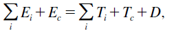(1)

where Ei and Ti are normative expenditure (expenditure needs) and tax revenue (tax capacity) of the n regional governments (i = 1...n), Ec and Tc normative expenditure and tax revenue of the central government, and D the deficit incurred by the central government. We assume for simplicity that Ec is all non-divisible public expenditure and Tc central government tax revenue whose regional origin is known. All variables are exogenous (normatively given) except D.

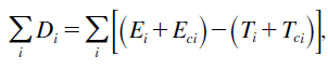
Rewrite (1) as follows:

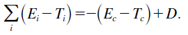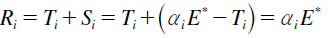
(2)

The left hand side of (2) shows the sum of the discrepancies between normative expenditure and tax revenue for the n regional governments. These discrepancies can be positive or negative depending on the particular relation between Ei and Ti. Suppose, for concreteness, that there exist a transfer system that equates fiscal capacity (EFC) (Musgrave, 1961; King, 1984). Under the EFC transfer system, the final amount of normative resources that region i will have at its disposal, Ri, is the sum of the region’s normative tax revenue, Ti, and the transfer it receives from the system, Si. That is,

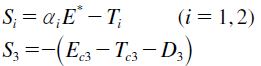
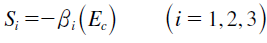
(3)

Si is defined as

(4)

and Ei, the normative expenditure of region i, is

(5)

where αi is the population share of region i, ai = Ni /N , and E* the aggregate of normative expenditure over all regional governments. Thus, as expression (6) shows, the amount of resources that the EFC system of transfers puts at the disposal of each region is αi E* :

(6)

Call the sum of Ri over all regions R*. Then, from (6)

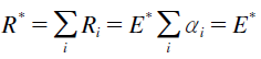
or

Consistently with the assumed balance of regional governments, normative re- sources are equal to normative expenditure.

Also from (6), dividing by Ni we have

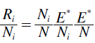
Thus, the EFC transfer system distributes total resources according to populationand thus equates the amount of resources per unit of need, Ri/Ni, toE*/N for allregions 1.

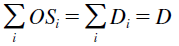
The sum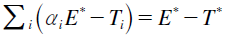 is the Vertical Fiscal Gap of the system, VFG,where T* is the total tax capacity of the regions, . The VFG measures theshortage between the total normative expenditure of the regions and their total taxcapacity, and formally can take the following different forms:

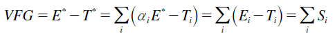(7)

If E* > T* , the aggregate net transfer goes from central to regional governments; and if E* < T* , from regional to central government.

2.2. Transfers between levels of government

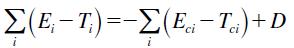
Expression (2) above is the basic relationship we will use to represent the trans fers that may exist between levels of government. Substituting (7) into (2) we have:

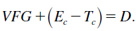(8)

The sum of the Vertical Fiscal Gap and the balance arising from the specific activity of the central government (that is, the balance before transfers to other Administrations) is equal to the public deficit of the economy. The left hand side of (8) measures the shortage (if it is positive) or surplus (if it is negative) of the economy. The right hand side, the public deficit of the economy, measures the increase in debt when there is a shortage or the decrease in debt when there is a surplus, which the economy will have to undertake.

We have assumed above that after the transfer system regions cannot have deficit. Thus the public deficit of the economy, D, must also be the public deficit of the central government considering not only its specific activity but also the management of the regional transfer system. Expression (8) is therefore the overall central govern ment budget, where net expenditures are Ec + VFG and tax revenue is Tc.

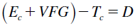
Ec is therefore the central government expenditure on the specific non-divisible public goods over which this Administration has responsibilities and excludes the net aggregate transfer to or from the regions. However, if we want to concentrate on the different flows of resources between levels of government, (8) is the appropriate form to use, where the VFG is the regional deficit, if positive, or regional surplus, if negative, and Ec - Tc is the central government specific deficit or the central government specific surplus. By specific we mean the central government balance excluding the VFG (that is, excluding transfers between levels of government).

The sign and magnitude of D will depend on the sign and magnitude of the VFG and the balance Ec - Tc . The VFG can be zero, positive or negative. If it is zero, the regional transfer system as a whole is balanced; that is, total normative expenditure is equal to total tax capacity, E* = T* . This does not necessarily imply that each individual region is balanced; it only means that if for some regions expenditure needs exceeds tax capacity, for others the opposite must be true and the sum of the positive regional transfers must equal the sum of the negative regional transfers. In this case we say that the regional transfer system is self-financed. If the VFG is positive, E* > T* , there is an overall regional deficit which must be financed with a transfer from the central government to the regions. And if the VFG is negative, E* < T* , there is an overall regional surplus which generates a transfer from the regions tothe central government. In our model all regional transfers are conducted through theintermediation of the central government.

Ec-Tc, the central government specific balance can also be zero, positive ornegative. If zero, central government specific expenditure equals tax capacity, Ec=Tc , and does not generate any additional financial claim. If positive/negative, (Ec > Tc) / (Ec < Tc), an additional central government specific deficit/surplus is also generated.

Table 1 shows the nine basic cases that result from the combination of these alternatives. It also shows that two of these nine cases, case 6 and case 8, generate three particular outcomes each. Thus, in total, we have thirteen possible cases.

Table 1.
Intergovernmental transfers and economy-wide public deficit. A map of alternatives

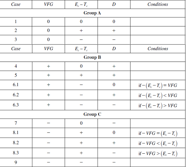
VFG: Vertical Fiscal Gap.

Ec - Tc: Central Government specific balance.

D: Economy-wide public deficit.

The first three cases, Group A, correspond to the three alternatives in which the regional transfer system is self-financed and are the easiest to analyse. Case 1 depicts a perfectly balanced economy. The regional transfer system is self-financed, VFG = 0, and the central government specific balance is also in equilibrium, Ec - Tc = 0 . Thus, using (8), the public deficit of the economy is zero, D = 0. There is no need of extra resources from the private sector (in addition to those obtained by taxation). And cases 2 and 3 are variants of case 1 with, respectively, a deficit and a surplus in the central government specific fiscal activity. Then the public deficit of the economy is equal to Ec - Tc , which means that the economy has a public deficit in case 2 and a public surplus in case ³. The second group, Group B, corresponds to those cases in which the regional transfer system generates a positive VFG. That is, the regional aggregate tax capacity is not sufficient to finance the aggregate amount of expenditure needs, E* > T* , and a transfer from the central government to the regions, equal to precisely the VFG, is needed. This is probably the most frequent case in actual transfer systems. Case 4 is complemented with an equilibrated specific central government balance, Ec - Tc = 0 , so the public deficit of the economy is the VFG, D = VFG. And case 5 considers a central government that generates an additional specific deficit, so the public deficit of the economy is the sum of the deficits of the two levels of government, D = VFG + Ec - Tc .

Case 6 contemplates a positive VFG and a negative central government deficit (that is, a central government surplus). These two opposite signs make the final effect on the public deficit of the economy dependant on the relative strength of the regional deficit and the central government surplus. The public deficit of the economy will be zero if the absolute value of the negative central government deficit is the same as the VFG, -(Ec - Tc) = VFG ; greater than zero if -(Ec - Tc) < VFG ; and less than zero if -(Ec - Tc) > VFG . These are respectively the cases 6.1, 6.2 and 6.3 shown in Table 1.

Finally, the third group, Group C, corresponds to the rather unusual situation in which the regions generate a negative VFG. This can only occur if the tax capacity ceded to the regions is sufficiently large relative to their expenditure needs so as to generate an aggregate negative VFG or, what is the same, an aggregate regional surplus. The cupo system applied in Spain to the Navarre and Basque Country regions would be relevant examples of this type of regional surplus.

Cases 7 and 9 are the easiest to analyse. In case 7, the regional surplus coexists with a balanced central government specific budget and therefore the public deficit of the economy is also negative and equal to the VFG, D = VFG. The economy as a whole generates a surplus and thus reduces its debt. In case 9 both levels of government gener ate a surplus, and thus the public deficit of the economy is also negative, and equal to the sum of the VFG and the central government specific surplus, D = VFG + (Ec - Tc).

Case 8, as case 6, combine two opposite signs: in this particular instance, a regionalsurplus and a central government specific deficit. The final effect on the publicdeficit of the economy depends on the relative strength of these two forces. The publicdeficit of the economy will be zero if the absolute value of the VFG is the sameas the central government specific deficit, -VFG=(Ec-Tc) ; greater than zero if-VFG < (Ec - Tc); and less than zero if -VFG > (Ec - Tc). These are respectivelythe cases 8.1, 8.2 and 8.3 of Table 1.

2.3. Regional redistribution. The measurement of pure redistribution

The above identifies the redistribution that goes on between levels of government, but not the redistribution of resources between regions. For that, in addition to the transfer system, we have to take into account the territorial incidence of the central government specific fiscal activity.

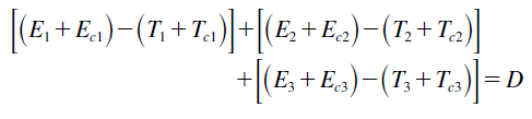
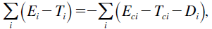
Under the assumptions of the model, both Ec and Tc can be either traced back or imputed to each of the n regions. So, from (2), disaggregating Ec and Tc into their regional components, we have:

(9)

or

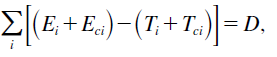(10)

where Eci is the central government expenditure located in or imputed to region i and is the central government revenue raised in region i and is the total public expenditure located and imputed to region i: expenditureundertaken by the own regional government plus that undertaken by the central government.Thus it makes sense to call this sum the total amount of public expenditurelocated or imputed to region i, Eti, where E E E ti = i + ci . Following a similar reasoning,the total amount of tax revenue obtained from region i is Tti=Ti+Tci . Therefore,using these two new definitions, the consolidated public constraint of the economy is:

(11)

where the difference Eti - Tti is the net overall transfer of region i, OSi. The difference Eit - Tit integrates both the effect of the EFC transfer and the fiscal activity of the central government.

If the public sector is balanced, , then the set of these overall transfers (which will normally be positive and negative) is sufficient to define the degree of pure redistribution going on in this economy. We call this, the degree of economy-wide pure redistribution.

Observe also that, since , (11) can be rewritten as follows:

(12)

from where it follows that:

(13)

The overall transfer of region i, OSi, is therefore both a measure of how the redistribution of resources affects region i, and a measure of the contribution of this region to the public deficit of the economy.

For simplicity, in this paper we will measure territorial redistribution at a public deficit of the economy equal to zero, D = 0. None of the results obtained below are affected by this assumption. All of them would follow for a positive (or negative) deficit. What is important, however, is that, in order to make the results of different scenarios strictly comparable between them, the level of D is the same in all our simulations. This must be so, particularly if we are interested in arriving at a quantitative measure of the degree of pure redistribution. The assumption D = 0 also, simplifies the presentation significantly. We will see below that not all cases we want to discuss are balanced; that is, not all scenarios end up with D = 0. When this situation arises, we impose the condition D = 0 and define the case so that, while maintaining the transfer systems under analysis, the above restriction is fulfilled. We illustrate this approach below, for the particular cases in which it is needed.

It is important to notice that when the public deficit is zero, necessarily the totalnormative expenditure of the economy —that is, the normative expenditure of theregions plus the normative expenditure of the central government— must be equalto the total tax revenue of the economy. This can be easily seen starting from expression(1). Let us call the total normative expenditure of the economy E —that is,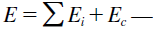and the total normative tax revenue T, where 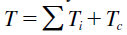. Thenexpression (1) reduces to E = T + D and if D = 0 it must be the case that E = T.

Finally, in addition to D = 0, in all cases, we also keep unchanged: i) the total normative expenditure of the economy; ii) the total tax revenue obtained (that is, we keep constant the tax effort of the economy), and iii) the regional distribution of tax capacity (that is, the regional distribution of income).

3. The model at work: centralized economy

3.1. Description of the economy

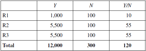
Following López-Laborda (2004), we consider an economy with three regions: R1, R2 and R3. As shown in Table 2, all regions have the same population, 100 in-habitants each. R1 is the least productive one, with 1,000 monetary units (mu) of output, while R2 and R3, 5.5 times more productive than R1, have an output of 5,500 mu each.

Table 2.
Economy’s data

3.2. Centralized economy

We explore first the extent of regional redistribution in the context of a centralized economy. This is not the purpose of the paper, but it will be useful as a bench- mark for the decentralized institutional settings that we explore below.

Suppose public expenditure is 10% of GDP. Half of it can be territorialized and is regionally distributed according to population, which is the measure of regional needs used by the Government. The other half corresponds to non-divisible government services, which for the purpose of the present exercise we assume it can be imputed to regions also in terms of population. The government revenue is also 10% of GDP, which is obtained by a proportional income tax, with a tax rate equal to 0.1.Therefore, the government runs a balanced budget.

What does the general analytical framework developed above has to say about the redistributive properties (if any) of this centralized economy?

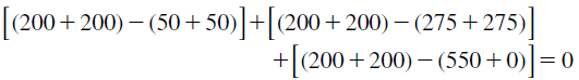
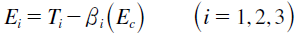
In this economy, by definition, there are no regional governments and thus Ti = Ei = 0 (i = 1,2,3). Therefore, expression (10) takes a very simple form that only involves the regional incidence of central government expenditure and tax revenue:

Under the above assumptions, Ec1 = Ec2 = Ec3 = 400 , Tc1 = 100 Tc2 = Tc3 = 550 . Therefore, the numerical version of (14) is:

(400 - 100) + (400 - 550) + (400 - 550) = 0

or

(15)

Table 3.
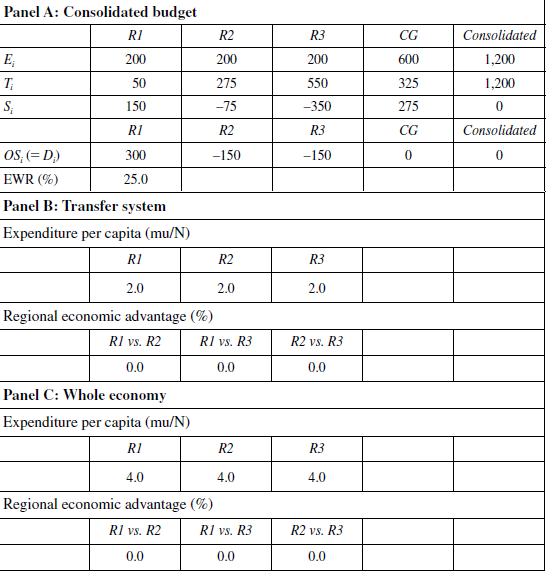
Centralized economy. Consolidated budget (Monetary units, mu)

D: Deficit; S: Regional transfer; OS: Overall transfers; EWR: Economy-wide redistribution.

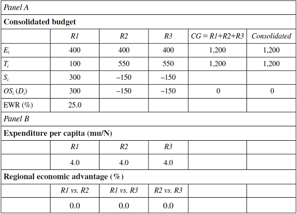
As Panel A of Table 3 shows, the central government runs a balanced budget, with D = Ec - Tc = 1, 200 - 1, 200 = 0 . Therefore, the three overall territorial transfers are necessarily self-financed, and the economy needs no additional finance from outside the public sector. The overall transfers to R1, R2 and R3 are, respectively, 300 mu, –150 mu and –150 mu. R1 is the net recipient of resources, for an amount of 300 mu, which can be thought of as financed by R2 and R3 to the tune of 150 mu each. In this scenario, the economy redistributes 300 mu out of a total amount of resources of 1,200 mu. The degree of economy-wide pure redistribution is therefore 25% [=(300/1,200)*100]. All regions have at their disposal 4 mu per unit of need. Under the assumptions here maintained, all regions are equally treated by the central (and only) government as far as the provision of public goods and services is concerned.

4. The model at work: decentralized economy

4.1. Equalization of Fiscal Capacity (EFC) transfer system

Suppose now that the economy is decentralized in the following manner. The total amount of divisible public expenditure, E* = 600, is the responsibility of three regional governments instituted in the three regions, and the central government takes responsibility of the non-divisible part of public expenditure, Ec = 600. Regarding normative tax revenue, regional governments are given half the tax capacity, which is defined by a proportional 5% tax on income that yields in total 600 mu(T* = 600), and the central government also taxes income by a 5% proportional rate, with Tc = 600. Thus the two levels of government are balanced and, for the aggregate of the three regional governments, the VFG is zero,

VFG = E* - T* = 600 - 600 = 0,

and so it is the central government specific balance,

D = Ec - Tc = 600 - 600 = 0.

This is precisely the Case 1 of Table 1, where there is full balance in all government levels of the economy. The transfer system is self-financed, the central govern ment is balanced and, therefore, the public deficit is zero.

Given the figures of regional income shown in Table 2, the three region’s normative tax revenue are as follows: T1 = 50 and T2 = T3 = 275. On the other hand, the three EFC regional transfers, Si = aiE* - Ti, are: Si = 200 - 50 = 150; and S2 = S3 = 200 - 275 = -75. Therefore, the normative expenditure of the three regions, Ei = Ti + Si, are: Ei = 50 + 150 = 200 and E2 = E3 = 275 - 75 = 200. After the operation of the EFC transfer system, all three regions, despite their different tax capacity, end up with sufficient resources, 200 mu each, to just finance their respective normative expenditure.

Table 4.
EFC transfer system (Monetary units, mu)

D: Deficit; S: Regional transfer; OS: Overall transfers; EWR: Economy-wide redistribution

The EFC transfer, Si = αiE* - Ti, may give the impression that regional governments have very little discretion in the management of their budget. But account must be taken that all the values considered here are normative values and that, depending on the manner in which expenditure and tax responsibilities are defined, actual levels of expenditure and tax revenue may differ from normative levels if these governments are prepared to apply a fiscal policy that differs from the normative one. In this paper we restrict ourselves to the analysis of transfers in normative terms. That is, we assume that regional governments and the central government do not deviate at all from their assigned normative levels of expenditure and tax revenue.

Regarding the regional incidence of the central government fiscal activity, under the assumptions here maintained, we have that Ec1 = Ec2 = Ec3 = 200 , Tc1 = 50 and Tc2 = Tc3 = 275 .

Differently from the case of the centralized economy, now the overall transfers are the consequence of both regional and central government effects. We thus take expression (10), which for the three regions described here reads:

And in numerical terms:

which reduces to

300 - 150 - 150 = 0.

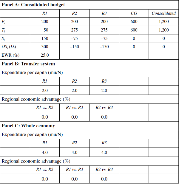
As in the centralized economy, a balanced decentralized economy with an EFC transfer system will display a set of overall transfers for R1, R2 and R3 respectively equal to 300 mu, –150 mu and –150 mu. Taking into account the fiscal activity of the regions and the central government, this scenario redistributes 300 mu out of a total of 1,200 mu. Therefore, the degree of economy-wide pure redistribution is 25% [=(300/1,200)*100], the same as that of the centralized economy. This is shown in Panel A of Table 4.

The EFC transfer system puts at the disposal of the three regions the same amount of resources per unit of need: 2 mu. And when the fiscal activity of the central government is taken into account, the result is, as in the centralized economy, 4 mu to each region. So a decentralized economy with an EFC transfer system has the same redistributive effects as a completely centralized economy, providing that in both cases the aims of the central government is to distribute resources among regions according to their relative needs (see Panels B and C of Table 4).

4.2. «Mixed Transfer System 1»: R1 and R2 under EFC, and R3 under an «equalizing special regime»

Zabalza and López-Laborda (2017) use their model not so much to identify measures of redistribution, but rather to exploit a duality result regarding the way in which transfers can be measured. In particular, we note that expression (10) abovecan be rewritten in the following manner:

(16)

or

(17)

Expression (16) gives directly the n regional components in which the total public deficit can be decomposed. And expression (17) provides the definition of the contribution of region i to the total public deficit.

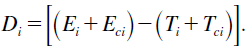
Given that , expression (9) can also be expressed as follows:

(18)

where Di is defined in (17). By construction the n parentheses on the left hand side of (18) are pairwise identical to the n parentheses on the right hand side. Then, given that by (4) the parentheses on the left hand side are the EFC transfers, it follows that these transfers can be defined either as the simple difference between the normative expenditure and tax revenue of the region, αiE* – Ti, or by the negative of an expression that measures the expenditure that the central government makes in the region, minus the tax revenue that it raises and the public deficit generated in this same region. Thus:

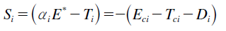(19)

The structure of the expression -(Eci-Tci-Di) , is the same as that of the Spanish«cupo» applied to the Basque Country and Navarre. The actual contents, however,is different as we shall see in the next section, where a «non-equalizing special regime» is analysed.

In the present scenario we use this duality result to define a mixed transfer system, which we call «Mixed Transfer System 1», composed, among other variations respect to the previous scenario, of the two alternatives offered by expression (19). Concretely, R1 and R2 remain under the EFC transfer system and an «equalizing special regime» is applied to R3. By «special regime» we mean that R3 is given a higher level of fiscal autonomy than R1 and R2. To simplify, suppose that R3 is given the whole tax capacity of the region, so that the Central Government does not raise any tax revenue in that territory. By «equalizing» we mean that despite this high tax capacity, and despite that the transfer is defined differently from that of R1 and R2, R3 ends up having the same resources per capita as those enjoyed by R1 and R2. Therefore, the two types of transfers of the «Mixed Transfer System 1» are:

(20)

Regarding tax revenue, R1 and R2 have the same levels as those of the previous scenario (Section 4.1), but R3 and CG change. Under the ECF system, R3 raised 0,05*5,500 = 275 and the CG raised in the R3 territory also 0,05*5,500 = 275. Now, R3 raises 0,1*5,500 = 550 and CG does not raise any tax revenue in R3 territory. There is a 275 mu shift in tax revenue out of GC and into R3, which does not alter the total tax revenue raised in the economy, that remains at 1,200 mu.

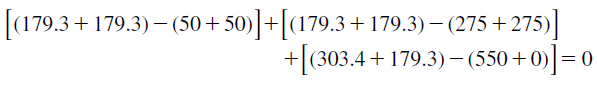
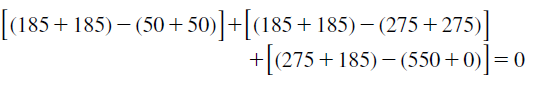
The transfers of R1 and R2 are the same EFC transfers of the previous scenario. Namely, the R1 transfer is 150 mu and that of R2 –75 mu. But the transfer of R3 is now given by the second expression of (20) and it is instructive to detail its calculation. Ec3 is one third (R3’s population share) of total central government expendi ture; that is (1/3)*600 = 200. Tc3 is zero, since under the new assumption, the central government does not raise any tax in R3’s territory. And following expression (17), and recalling that under the new assumption R3 collects all taxes in its territory, D3 is –150 mu [= (200 + 200) – (550 + 0)]. This makes S3 = -(200 - 0 + 150) = -350 mu. The «equalizing special regime» transfer is such that the expenditure that R3 can finance, E3 = T3 + S3, is the same as that of R1 and R2 with their EFC transfers despite its larger tax capacity and the different formula of its transfer. Indeed, with the «Mixed Transfer System 1» the normative expenditure of the three regions are: for R1,E1 = 50 + 150 = 200; for R2, E2 = 275 - 75 = 200; and for R3, E3 = 550 - 350 = 200.

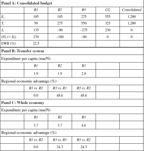
As Panel A of Table 5 shows, an important difference between the present «Mixed Transfer System 1» and the previous EFC transfer system is that while the latter is self-financed (it corresponds to case 1 in Table 1), the former generates an important negative VFG; that is, an important positive transfer for the central government (it corresponds to case 8.1 in Table 1). The three R1, R2 and R3 transfers are, respectively, 150, –75 and –350. This sums –275. The regional system as a whole contributes to the central government 275 mu. With this, R2 and R3 compensate the central government; R2 for the excess tax capacity over its normative expenditure, and R3 also for the 275 mu higher tax capacity that this particular transfer system bestows on this region.

Table 5.
Mixed transfer system 1* (Monetary units, mu)

* R1 and R2 under EFC transfers, and R3 under an «equalizing special regime» transfer.

D: Deficit; S: Regional transfer; OS: Overall transfers; EWR: Economy-wide redistribution.

It is precisely this positive transfer what allows the central government to complement its remaining 325 mu tax revenue, in order to finance the 600 mu expenditure needs it has. So, we have a scenario in which the public sector is balanced overall, thanks to the existence of a sizeable vertical transfer between the two levels of government. Panel A of Table 5 shows the budget of the three regions, that of the central government and the consolidated budget of the whole economy.

We turn now to the evaluation of the overall set of transfers, so that the degree of pure redistribution of the whole economy can be assessed. In the present scenario, expression (10) yields the following numerical form:

where, as compared with the previous scenario, we note the difference of the last pa renthesis due to the cession to the regional government R3 of the whole tax capacity of the region. Despite this difference, the final overall set of transfers turns out to be the same as that of the EFC transfer system:

300 - 150 - 150 = 0

Therefore, we conclude that the degree of pure redistribution of the «Mixed Transfer System 1» is the same as that of the EFC transfer system; namely, 25% [=(300/1,200)*100].

Despite the negative VFG generated, Panel B of Table 5 shows that this scenario puts at the disposal of all the regions 2.0 mu per unit of need, and Panel C that when the fiscal activity of the central government is considered, this figure increases to 4.0 mu per unit of need. So, as it is the case with the EFC transfer system, the «Mixed Transfer System 1» distributes resources equally among regions.

In this exercise we do not enter into the efficiency cost of the different systems of transfers. In fact we assume away any such cost. But if the implementation of transfers, even between different government levels, involves the consumption of resources (e. g., costs of negotiation, unjustified delays, increased auditing costs), then the mixed system of transfers examined in this section would be more expensive to run than the EFC transfer system due to the sizeable vertical transfer from the regional to the central levels of government (275 mu). This suggests that placing the whole tax capacity in the regional level, which is the defining characteristic of the «special regime», may not be a reasonable course of action. We believe that tax decentralization improves the fiscal responsibility and autonomy of the regions, but it is difficult to justify that the extent of this decentralization should go further than the limit set by their total normative expenditure.

4.3. «Mixed Transfer System 2»: R1 and R2 under EFC, and R3 under an «non-equalizing special regime»

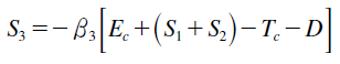
Suppose now that the situation is the same as that discussed in the previous case,only that now R3, instead of paying the «equalizing special regime» transfer representedby expression (20), pays a significantly smaller transfer, which we call the«non-equalizing special regime» transfer. This lower or «non-equalizing special regime» transfer is defined as follows:

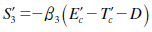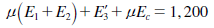
(21)

The «non-equalizing special regime» transfer has the same structure as the «equalizing special regime» transfer defined in expression (20) but with significant differences, that are meant to represent the real cupos that are applied to the two Spanish foral communities —Basque Country and Navarre—. The first one is that the three elements within the parenthesis of (21), central government expenditure, central government tax and central government deficit, rather than being directly referred to the R3 territory, are referred to the national equivalent of those items. Second, the measurement of Ecl is the specific expenditure of the central government budget minus the expenditure in that budget that corresponds to responsibilities ceded to R3. In our particular example, since there is a clean division between territorialized expenditureand non-divisible expenditure, and the central government only has responsibilitiesfor non-divisible expenditure, the central government expenditure does notinclude any expenditure that corresponds to the responsibilities ceded to R3. Therefore,in our model, Ecl is equal to Ec. Third, Tcl is the amount of revenue obtainedby the central government with those taxes not ceded to R3. In our model, to makethings extreme and more visible, we have assumed that under this «special regime»all taxes have been ceded to R3. Therefore, in the central government budget there isno revenue coming from taxes that have been not ceded to R3, so Tcl= 0 . Fourth, thedeficit of the economy (that is, the deficit of the Central Government) must be zeroto ensure the comparability of results. And fifth, the national equivalents that appearwithin the parenthesis of (21) are scaled down to the dimension of R3 by multiplyingthis parenthesis by an imputation coefficient that we take it to be the R3 tax capacityshare,β3². As we shall presently see, with (21), which under the particular conditionsdescribed above reduces to

(22)

R3 has a negative transfer of lower absolute value than with the «equalizing spe cial regime» transfer (20). That is, R3 has to pay a lower «cupo», to use the terminology of the foral Spanish system.

If it pays a lower cupo, R3 will have more resources to spend and, other things equal, the deficit of the economy will increase. This poses two problems. The first is that, as pointed out above, with a positive deficit a figure for the degree of redistribution strictly comparable to those obtained in previous exercises cannot be found. The second is that the assumption that everything else remains the same can hardly be sustained. So we must find an approach so that the operation of these two transfer systems is constrained to a zero public deficit. Since what we are interested in is the study of territorial redistribution as a result of different transfer systems, the most natural assumption to make is to distribute the absorption of the excess of resources assigned to R3 equally, in proportional terms, between R1, R2 and CG. By doing this, while we reduce the resources available to these three jurisdictions, we keep constant their relative needs.

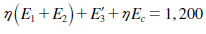
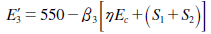
Call n (0 < n < 1) the common multiplicative factor that reduces the normative expenditure of R1, R2 and CG so that D = 0. Then, if E1, E2 and Ec are the initial levels of normative expenditure (200 mu, 200 mu and 600 mu respectively) it must be the case that

(23)

where

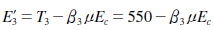(24)

We can easily find the reduction required by substituting (24) into (23) and solv ing for n to obtain

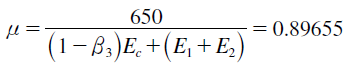
The effort that R1, R2 and CG have to make in order to absorb the increase in the expenditure of R3 is (1 - n) per cent; that is, a 10.345% reduction of their respective levels of normative expenditure.

Table 6 presents the results of this new scenario. As postulated, the normative expenditure of R1, R2 and CG is 10.345% lower than in the equalizing «Mixed Transfer System 1» shown in Table 5, and the public deficit is zero. Also, it is easy to verify that the non-equalizing transfer of R3, expression (22), yields the –247 mu figure shown in the table, significantly lower (in absolute terms) than the –350 mu of Table 5. The «cupo» of R3 is therefore much more generous to R3 than the one that would yield equality, and therefore the expenditure of R3 raises from 200 mu to 303 mu. This excess is financed with lower transfers for R1 and R2 (129 mu and –96 mu versus 150 mu and –75 mu in Table 5) and with the lower vertical transfer that the CG receives (213 mu versus 275 mu in Table 5).

Regarding the overall transfers, the numerical form of expression (10) for this particular scenario is:

or

258.6 - 191.4 - 67.2 = 0

Therefore, the degree of pure redistribution of the «Mixed Transfer System 2» is 21.5% [(=258.6/1,200)*100]. As would be expected from the equalizing nature of the «Mixed Transfer System 1» scenario, the redistributive potency of the non- equalizing «Mixed Transfer System 2» scenario is significantly lower. It goes down from 25.0% to 21.5%.

Table 6.
Mixed Transfer System 2* (Monetary units, mu)

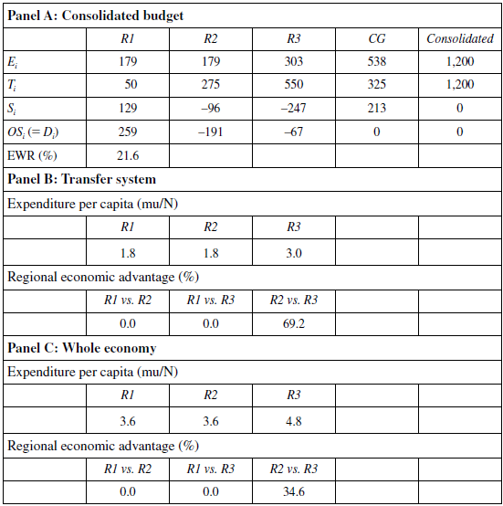
* R1 and R2 under EFC transfers, and R3 under a «non-equalizing special regime» transfer. D: Deficit; S: Regional transfer; OS: Overall transfers; EWR: Economy-wide redistribution.

Finally, Panels B and C report the amount of resources per unit of need that each re gion enjoys after respectively the consideration of only the mixed transfer system (Panel B) and the consideration of both the transfer system and the central government fiscal activity (Panel C). As Panel B shows, the strong non-equalizing nature of the present particular mix puts at the disposal of R3 3.03 mu per unit of need compared with only 1.79 mu for R1 and R2, thus generating an economic advantage of R3 versus R1 and R2 of 69.2% 3. Things improve somewhat after considering the additional fiscal presence of the central government. Then, as indicated in Panel C, the comparison between R3, on the one hand, and R1 and R2, on the other, is 4.83 mu per unit of need versus 3.59 mu per unit of need, and economic advantage of R3 respect the other two regions of 34.6%.

4.4. R1, R2 and R3 under an «equalizing special regime»

From Section 4.2 we know that the transfer generated by the «equalizing» special regime is exactly the same as that of the EFC system. One would be excused to think that, because of this fact, there is no need to consider the case in which all regions are under the «equalizing special regime» because its results must be identical to the case in which all regions are under the EFC transfer system, which has already been considered in Section 4.1. However, this is not quite so because the «special regime», in comparison with that of the EFC system, moves a certain degree of tax capacity from the central government to the regional governments. To see what is going on more clearly, and consistently with what we have assumed for R3, we make here the extreme assumption that all fiscal capacity is ceded to all the three regional Governments, thus leaving the central government with no tax revenue of its own and totally dependent on the transfers coming from the regions to finance its expenditure responsibilities. Therefore, the three regions tax their respective base at a 10% rate: R1 obtains 100 mu, and R2 and R3, 550 mu each.

The three «equalizing» transfers that correspond to this case are:

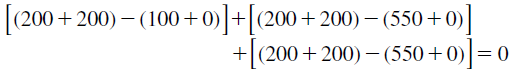
(25)

Under the maintained assumptions, . And the contributions of the three regions to the public deficit of the economy are obtained evaluating numerically expression (12):

D₁ = (200 + 200) - (100 + 0) = 300

D₂ = (200 + 200) - (550 + 0) = - 150

D₃ = (200 + 200) - (550 + 0) = - 150

Then, substituting these values into (25) we obtain the three «equalizing» trans fers of this case:

S₁ =-8200 - 0 - (300)B = 100

S₂ =-8200 - 0 - (- 150)B = - 350

S₃ =-8200 - 0 - (- 150)B = - 350

Using all this information, Panel A of Table 7 presents the consolidated budget of the economy. Normative expenditure turns out to be 200 mu for all three regions: A system with an «equalizing special regime» transfer for all regions gives exactly the same results as those of the EFC system of transfers of Section 4.1. However, when we compare Tables 7 and 4, we see that the form in which these same final results are obtained differ significantly. The main difference is that under the «special regime» the central government is left with no resources of its own, so that a net aggregate transfer from the regions of 600 mu is needed for that level of government to finance its expenditure responsibilities. And this is precisely the end to which the three «equalizing» transfers are directed. R1 still has a positive transfer (that is, it obtains money from the system), even if smaller than the one of the EFC system (100 versus 150 mu). And R2 and R3 have a negative transfer (that is, they pay money to the system) of a much larger absolute value than in the case of the EFC mechanism (–350 versus –75 mu each). In total, then, the system of transfers provides a vertical transfer to the central government of 600 mu (= -100 + 350 + 350) with which to finance its expenditure responsibilities. This scenario is also an example of case 8.1 in Table 1: a negative FVG of equal absolute value as the specific deficit of the central government, the excess of Ec over Tc.

Table 7.
All regions under «equalizing special regime» (Monetary units, mu)

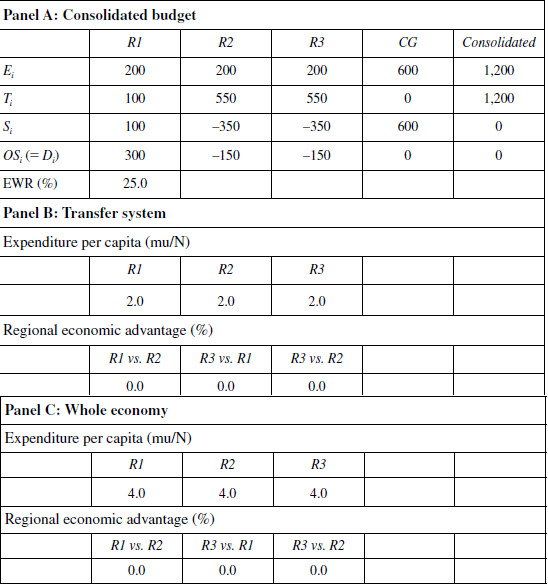
D: Deficit; S: Regional transfer; OS: Overall transfers; EWR: Economy-wide redistribution.

Taking now into account the added effect of the fiscal activity of the central government, we find that the numerical form of expression (10) is:

or

300 - 150 - 150 = 0

This is exactly the set of overall transfers of the EFC transfer system and there-fore the degree of pure economy-wide redistribution is also 25% [=(300/1,200)*100].

Panels B and C confirm that the results regarding the amount of resources per unit of need is the same for all regions, both after the transfers system, and under the joint effect of the transfer system and the fiscal activity of the central government. As we would expect given that this system has the same effects as the EFC system, all region are equally treated. There is no economic advantage for any of them. The only difference with respect to the EFC transfer system is the huge negative VFG that the present scenario generates, due to the cession of all the tax capacity to the regions.

4.5. R1, R2 and R3 under the «non-equalizing special regime»

In this section we consider the case in which the «non-equalizing special regime» is generalized to all regions. This means that the three regions have all the tax capacity of the economy and the tax revenue of the central government is zero. Then, if to make this case comparable with the previous ones, the public deficit has to be zero, D = 0, knowing that the whole of this deficit is generated in the central government, it must be the case that the negative of the VFG —that is, the negative of the sum of the three regional transfers— must be equal to the specific expenditure of the central government, -VFG = Ec. This again is a scenario that corresponds to Case 8.1 in Table 1 for Tc = 0.

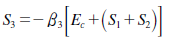
Since the public deficit of the economy is zero and the central government raises no taxes in the regions, generalizing expression (21) we see that the transfers of the three regions take all of them a very simple form, namely:

Therefore, normative expenditure, Ei = Ti + Si, is:

In numerical terms:

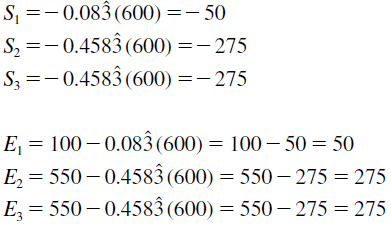
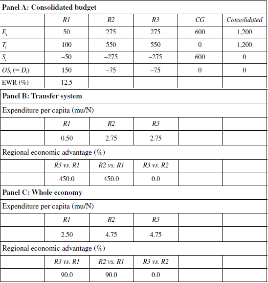
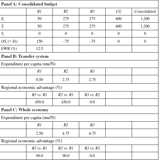
Panel A of Table 8 shows that under the «non-equalizing special system», since all the tax capacity is ceded to the regions, all three of them, including R1, the poor one, have to contribute to the finance of the 600 mu expenditure of the Central Government. With the corresponding transfers, the Central Government can finance its expenditure responsibilities (50 + 275 + 275 = 600), and its public deficit, which is also the consolidated deficit of the economy, is zero. In terms of the amount of normative expenditure that the system assigns to the regions, R1 is left with only 50 mu while R2 and R3 have 275 mu each. See that the regional distribution of normative expenditure follows exactly the distribution of tax capacity: R2 and R3 have 5.5 times more resources than R1, which is exactly the ratio in which the productivity of R2 and R3 stands with respect to the productivity of R1.

Table 8.
All regions under «non-equalizing special regime» (Monetary units, mu)

D: Deficit; S: Regional transfer; OS: Overall transfers; EWR: Economy-wide redistribution.

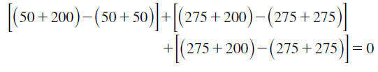
The overall transfers of this economy —expression (10)— are:

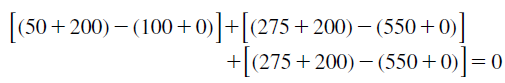
or

150 - 75 - 75 = 0

In net terms the taxpayers of R2 and R3 contribute 75 mu each to finance a net transfer of 150 mu in favour of R1. A degree of pure redistribution of 12.5% [= (150/1,200)*100], half the size of that obtained with the «equalizing special regime» for all regions considered in the previous section.

As Panels B and C show, the final amount of expenditure per unit of need that this system assigns to R1 is particularly low: 0.5 mu per capita, as compared with 2.75 mu per capita each that R2 and R3 obtain; an economic advantage of R2 and R3 over R1 of 450%. As it happens with the totals examined above, resources per capita are 5.5 times greater in R2 and R3 than in R1; normative expenditure per capita is fully guided by regional relative productivity. After the intervention of the central government budget, this inequality is somewhat mitigated: R1 has 2.50 mu per unit of need, as compared with 4.75 mu for R2 and R3. Now the economic advantage of these two regions is reduced to 1.9 times, which means that they still enjoy 90% more resources per capita than R1.

The two «special regimes» considered in this paper, one of which —the «non- equalizing» variety— is an approximation to the actual way in which the two Spanish foral communities are financed, cannot be generalized without causing havoc among the great majority of the Spanish autonomous communities. And for the same reason, they cannot be extended to other rich communities such as Madrid and Catalonia. Also, there is no point in having a system which leaves the central government without direct means to finance the non-divisible services of which it is responsible, particularly when some of them (for instance, macroeconomic management) may need resources at short notice and in volumes not foreseen in the normative design of the transfer system. And finally, it is absurd that the level of government that, on occasions and unexpectedly, may need to incur in considerable amounts of debt, is deprived of the capacity to tax the fiscal base of the economy.

4.6. A «Pseudo Equalizing Special Regime»

The significant economic advantage that the «non-equalizing special regime» has over the EFC transfer system in the «Mixed Transfer System 2» has in the past elicited proposals to eliminate, or at least mitigate, this advantage by making the beneficiaries to participate in the financing of the VFG of the regions under the EFC system. Regarding the Spanish «foral» system and, in particular, the advantage that the Basque Country and Navarre enjoy over the other Spanish regions under the «com- mon» system, these proposals have been discussed, for example, in Sevilla (2001), Castells et al. (2005), Monasterio (2009) and de la Fuente (2011).

In terms of our model this means that the transfer of the «non-equalizing special regime» (21) has to be redefined as follows:

which, given the assumptions of this particular case, Tc = 0 and D = 0, reduces to

(26)

Two initial comments worth considering are the following:

First: If the purpose is to eliminate the economic advantage of R3, there is a much more direct and effective way of achieving this goal by adopting the «equalizing special regime» that we have presented above in Section 4.2. It is possible to have a mixed transfer system in which some regions operate under the EFC system and others under a «special regime» that concedes much larger tax autonomy to the regions, and that allows to calculate the transfer in the indirect manner of expression (20). And we have shown that, despite fulfilling all these particularities, such mixed system (the «Mixed Transfer System 1») would deliver exactly the same results as those of a straight EFC system for all regions.

And second: The proposal reflected in (26) defines the transfer to one particular region in terms of the transfers of the rest of the regions, which is odd in terms of the concept of transfer. A set of transfers is a system that corrects for some under- ling disequilibrium between expenditure and revenue. Therefore the definition of a transfer is bound to be closely linked to the particular disequilibrium that needs to be corrected, not to other discrepancies in the system.

As in Section 4.3, we note that if R3 obtains through (26) more resources than the ones associated to the equalizing special transfer, and we want to keep the public deficit of the economy at zero, then R1, R2 and CG will have to compensate for this increase accepting a decrease in its normative expenditure. We make here the same assumption as that employed in Section 4.3: we distribute the absorption of the excess of resources assigned to R3 equally, in proportional terms, between R1, R2 and CG. So, while we reduce the resources available to these three jurisdictions, we keep constant their relative expenditure needs.

Calling now h(0 < h < 1) the multiplicative factor that reduces the normative expenditure of R1, R2 and CG, if E1, E3 and Ec are the initial levels of normative expenditure it must be the case that

(27)

where

(28)

and

(29)

(30)

Substituting (29) and (30) into (28) and the resulting expression into (27), and solving for h we obtain

The effort that R1, R2 and CG have to make in order to absorb the increase in the expenditure of R3 is (1 - h) per cent; that is, a 7.5% reduction of their respective levels of normative expenditure.

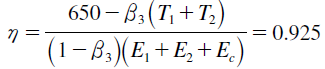
Table 9 presents the results of the «Pseudo Equalizing Special Regime» (PESR). The normative expenditure of R1, R2 and CG is 7.5% lower than in the equalizing «Mixed Transfer System 1» shown in Table 5, and the public deficit is zero. Also, it is easy to verify that the non-equalizing transfer of R3, calculated ac- cording to expression (26) with the adjusted values of Ec, S1 and S2, is effectively –275 mu 4. As in Section 4.3, the transfer of R3 is lower in absolute terms than the one that would yield equality and therefore the expenditure of R3 increases from 200 mu to 275 mu. This excess is financed with lower transfers for R1 and R2 (135 mu and –90 mu versus 150 mu and –75 mu in Table 5) and with the lower negative VFG that the CG receives (230 mu versus 275 mu in Table 5). We are again in Case 8.1 of Table 1.

Regarding the overall transfers, the numerical form of expression (10) for this particular scenario is:

or

270 - 180 - 90 = 0

Therefore, the degree of pure redistribution of the «PESR» system is 22.5% [(= 270/1,200)*100].

Table 9.
«Pseudo Equalizing Special Regime» (Monetary units, mu)

* R1 and R2 under EFC transfers, and R3 under a «pseudo-equalizing special regime» transfer.

D: Deficit; S: Regional Transfer; OT: Overall transfers; EWR: Economy-wide redistribution.

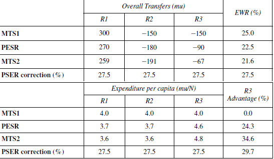
How do these results compare with those of the «Mixed Transfer System 2» scenario? We answer this question with the help of Table 10, where the systems MTS2 and PESR are compared regarding the pattern, across the three regions, of the overall transfers and the levels of expenditure per capita. For reference purposes, the table also includes the scenario MTS1 in which R3 has the equalizing special regime transfer (and R1 and R2 the EFC transfer) and full equality is achieved.

Table 10
MTS2 and PESR: Performance compared

MTS1: R1 and R2 with EFC transfers; R3 with equalizing special regime transfer. PESR: Pseudo Equalizing Special Regime.

MTS2: R1 and R2 with EFC transfers; R3 with non-equalizing special regime transfer.

The PESR corrects the unequal pattern resulting from MTS2, but the correction is incomplete if we take as reference the egalitarian pattern associated to MTS1. Regarding overall transfers, and with respect to the values of MTS2, the PESR increases those of R1 and R2 and decreases that of R3, thus moving as expected towards the egalitarian pattern of MTS1. However, out of the whole difference between MTS1 and MTS2, the PESR only covers 27.5% of it. The same occurs with the Economy- Wide Redistribution index: with respect to MTS2, the PESR increases pure redistribution from 21.6% to 22.5%; but this only represents 27.5% of the whole distance between MTS2 and MTS1. Regarding expenditure per capita, and again with respect to MTS2, the PESR reduces the R3 economic advantage over R1 and R2 from 34.6% to 24.3%, but the levels of expenditure per capita of R1 and R2 are still below those of the equal distribution of MTS1. The PESR reduces by almost 10 percentage points the advantage of R3, but as shown by the MTS1 row equality of expenditure per capita is achieved when this advantage is zero. So the PESR covers only 29.7% of the total reduction needed to achieve equality.

In the context of the Spanish regional finance models, in which R3 enjoys the «non-equalizing special regime transfer», this exercise shows clearly the limitations of the PESR solution: the fact that R3 shares in the financing of the cost of the equalization applied to the other two regions, does not imply that full regional equalization is achieved. As noted by Castells et al. (2005), sharing in the cost of equalization and achieving equalization are different things. So we reiterate the conclusion that has been advanced above: if for whatever reason the «special regime» transfer is the desired system for some regions, full territorial equality can only be obtained if the «equalizing» variety of this transfer, presented in Section 4.2 above, is the adopted one.

5. Concluding remarks

In this paper we have presented a conceptual framework to analyse the redistribu- tive impact of transfers in the context of a decentralized economy, and have illustrated the use of this framework to analyse the distribution properties of a variety of transfer systems applied to a given economy numerically described, divided in three regions and with two levels of government —the central level and the regional level—. For this purpose, we have used as benchmark the redistribution going on in a centralized economy, in which tax capacity is unevenly distributed across the three regions and central gov- ernment public expenditure is distributed across regions according to their population.

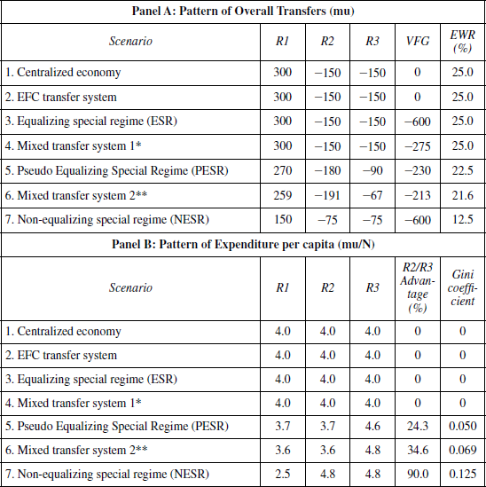
It is useful to review the numerical results obtained with the help of Table 11, where in Panel A we consider explicitly the overall transfers, the vertical fiscal gap, and the degree of economy-wide redistribution of the transfer systems analysed; and in Panel B the regional distribution of public expenditure per capita and the degree of economic advantage that some regions may have with respect to others. In or- der to make the results comparable, all transfer systems have been analysed holding

Table 11.
Comparison of different systems

VFG: Vertical Fiscal Gap: EWR: Economy Wide Redistribution.

* R1 & R2 under EFC; R3 under ESR** R1 & R2 under EFC; R3 under NESR.

constant the tax revenue and the level of normative expenditure of the economy, the distribution of tax capacity across regions, and the public deficit of the economy that in all cases is kept equal to zero. Holding the public deficit equal to zero, the transfer systems considered must necessarily fall within Cases 1, 6.1 and 8.1 of Table 1. The ones particularly considered in Table 11 belong to Cases 1 and 8.1. Although not explicitly shown, however, we also discuss below the nature of scenarios that pertain to Case 6.1.

Table 11 orders the scenarios according to their degree of economy wide redistribution (EWR). As compared with the 25% benchmark of the centralized economy, all scenarios either keep the degree of redistribution unchanged or reduce redistribution down to 12.5%, half the level of the benchmark. There are three transfer systems which according to the degree of EWR are undistinguishable from the benchmark: the EFC transfer system, the Equalizing Special Regime and the Mixed Transfer System 1. Their overall transfers are exactly the same as those of the centralized economy (300 mu are redistributed from the two rich regions, R2 and R3, which contribute 150 mu each, to the poor region R1). These transfer systems replicate the assumed territorial incidence of the centralized economy and, as shown in Panel B, yield a complete egalitarian economy as far as the territorial incidence of public expenditure per capita is concerned. No region has an economic advantage over any other. A significant difference, however, concerns the sizeable Vertical Fiscal Gaps of the Equalizing Special Regime (ESR) (–600 mu) and the Mixed Transfer System 1 (MTS1) (-275 mu). In both cases, in comparison with the EFC transfer system, the tax capacity of the three regions (ESR) or of one of the three regions (MTS1) is substantially increased at the expense of that of the central government. And this circumstance compels the generation of a significant positive transfer to the central government to enable this Administration to finance its public expenditure

The distinctive feature of the last three scenarios is that, as compared to the benchmark, they increasingly reduce the degree of redistribution, and render more unequal the distribution of regional public expenditure. As the last column of Panel B shows, while the Gini coefficient of the first four systems is zero (full equality), that of the last three systems increases from 0.05 for the Pseudo Equalizing Special Regime, to 0.125 for the Non-equalizing Special Regime. The more unequal effect of these transfer systems can be directly traced from the way in which the overall transfers and the level of expenditure per capita change.

Table 12
Gains (+), Losses (-) from full equality (Percentages)

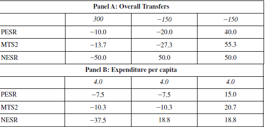
Sign indicates whether region losses (-) or gains (+).

PESR: Pseudo Equalizing Special Regime.

MTS2: Mixed Transfer System 2: R1 & R2 under EFC; R3 under

NESR. NESR: Non-Equalizing Special Regime.

This can be seen more clearly in Table 12, which, with respect to full equality, shows the gains and losses that each transfer system imparts on overall transfers (Panel A) and expenditure per capita (Panel B). Looking first at overall transfers, the table shows that all systems consistently reduce the overall transfers of R1 (the poorest region) and increase those of R3 (the richest region). Of particular interest are the effects of the Mixed Transfer System 2, which is patently designed to favour R3 in detriment of R1 and R2. The same conclusions follow from Panel B regarding the changes in expenditure per capita. In this case, the figures of the table are even easier to interpret than those of panel A to the extent that (allowing for rounding errors) for each system the sum of the three changes is zero, thus highlighting the strict redistributive character of the present exercise. In addition to the constraint of a zero public deficit, this paper has dealt only with transfer systems that generate either a zero or a negative Vertical Fiscal Gap. In particular, it has dealt with Cases 1 and 8.1 of Table 1. Had we considered, for each of the transfer systems, a lower assignment of tax capacity to the regions, we would have entered in the Case 6.1 of Table 1. We do not present these results here because there is not much to report about them. In- deed, whatever the transfer system, a reduction in the tax capacity of the regions (and thus an increase in the tax capacity of the central government) is completely neutral regarding the redistribution effects obtained here.

As explained above, the scenarios developed in this article are useful to better understand the distributive effects of regional finance in Spain and the differences that exist between the common and foral systems. Fundamentally, the common sys- tem of regional finance is based on the equalisation of fiscal capacity model (EFC), while the foral system is based on the non-equalizing special regime (NESR). The differences among them are clearly presented in the tables above. The exercise also considers several scenarios that help to visualize more clearly how the common and foral systems can be approximated while maintaining the distributive properties of the centralized economy, such as the application of the equalizing special regime to some regions (ESR) or to all of them (MTS1). Finally, the article explains why an alternative method proposed in the literature to approximate the foral to the common finance system, such as the pseudo-equalizing special regime (PESR), is less adequate.

References

Castells, A., Sorribas, P., and Vilalta, M. (2005): Las subvenciones de nivelación en la finan- ciación de las comunidades autónomas: Análisis de la situación actual y propuestas de reforma, Barcelona, Publicacions i Edicions de la Universitat de Barcelona.

De la Fuente, Á. (2011): «¿Está bien calculado el cupo?», Moneda y Crédito, 231: 93-167.

Fox, W. F. (2007): «The United States of America», in A. Shah (ed.), The practice of fiscal federalism: comparative perspectives, Montreal & Kingston, McGill-Queen’s University Press, 345-369.

King, D. (1984): Fiscal Tiers. The Economics of Multilevel Government, London, Allen and Unwin.

López-Laborda, J. (2004): «Financiación y gasto público en un Estado descentralizado», Eco- nomía Aragonesa, 24: 63-81.

Monasterio, C. (2009): «Un análisis del sistema foral desde la perspectiva de la teoría del federalismo fiscal», in C. Monasterio and I. Zubiri, Dos ensayos sobre financiación autonómica, Madrid, FUNCAS, 165-249.

Musgrave, R. A. (1961): «Approaches to A Fiscal Theory of Political Federalism», in Univer- sities-National Bureau Committee for Economic Research (ed.), Public Finances, Needs Sources, and Utilization, Princeton, NJ, Princeton University Press and National Bureau of Economic Research, 97-133.

Sevilla, J. V. (2001): Las claves de la financiación autonómica, Barcelona, Crítica.

Zabalza, A. (2018): «El mecanismo de nivelación de la financiación autonómica», Hacienda Pública Española/Review of Public Economics, 225: 79-108.

Zabalza, A., and López-Laborda, J. (2017): «The uneasy coexistence of the Spanish common and foral regional finance systems», Investigaciones Regionales/Journal of Regional Re- search, 37: 119-152.

ANNEX

Maximum to minimum redistribution via a parametric system of transfers

In this Annex we illustrate how the conceptual framework can be applied to mo els developed independently from the present exercise. In particular, we apply it to the parametric system of transfers presented in Zabalza (2018), which is capable of generating a continuous range of redistributive effects.

In the context of the discussion about the degree of equalization, Zabalza (2018) argues that if inequality is desired, is best to be transparent about it and suggests a parametric system of transfers which can generate any degree of equalization. This is achieved by making the degree of equalization to depend on a parameter that miti gates the potency of the horizontal transfers associated to the canonical EFC model. A subjective parameter that is both explicit and political.

In this Annex we show how the «non-equalizing special system» of Section 4.5 can be replicated in terms of this parametric model. This offers an alternative which is not only simpler, but also more susceptible of application since one of the most cumbersome features of the «special systems», namely the cession of all (or of a significant part of) the tax capacity to the regions, is not needed at all.

Given the assumptions of our decentralization model, the transfers of the three regions are given by the following expressions (adapted from Zabalza, 2018, p. 102, expression 26):

(A.1)

where E/2 and T/2 are the total normative expenditure and normative tax revenue as- signed to the three regions, t is the political parameter, a is the index of expenditure needs (which as discussed in Section 2.1, we measure by relative population), and b is the index of tax capacity (which as discussed in Section 4.3, we measure by relative normative tax revenue).

If t = 1, then from (A.1) the transfers are:

S1 =α1 (E/2) - b1 (T/2) (i = 1, 2, 3)

which are the transfers of the EFC model that generate total equality of resources per unit of need. This can be seen more easily looking at the amount of normative expen diture that the system assigns to the region, which equals the sum of the normative tax revenue and the transfer E_i = T_i + S_i, which for the above S_i reads:

E₁ = b₁ (T/2) + 8α₁ (E/2) - b₁ (T/2)B =α₁ (E/2)

(i = 1, 2, 3)

The normative expenditure assigned to the regions is distributed according to needs. There is complete equalization (as in Australia). This is exactly the EFC trans fer system discussed in Section 4.1 and will not be repeated here.

If t = 0, then we go to the opposite end of the range of redistribution. Using (26) and recalling that for D = 0, T = E, the transfers are zero for all regions:

S₁ =α₁ (E/2) -α₁ (T/2) = 0 (i = 1, 2, 3)

and the normative expenditure assigned to the regions is totally determined by tax revenue:

E₁ = b₁ (T/2) (i = 1, 2, 3)

As far as the system of transfers is concerned, there is no redistribution at all. Each region spends according to the tax revenue it normatively collects (as it happens, for example, in the USA) 5. This is the result obtained in Section 4.5, where we analyse the effects of a system in which all regions are under the «non-equalizing special regime» transfers. However, as we shall see, there is an important difference that justifies the explicit consideration of this particular model: whereas the «non-equalizing special regime» system requires the displacement of a huge amount of fiscal capacity between the two levels of government (from central to regional level), the parametric model with t = 0, achieves the same final outcome without such displacement.

Table A.1 presents the results of the parametric model with t = 0. The final results are exactly the same as those shown in Table 8 for the «non-equalizing special regime» for all regions. However, the present model does not displace half the tax capacity of the nation from the central government to the regional governments, and thus avoids the need to generate negative transfers (cupos) so that the central govern- ment can finance its expenditure responsibilities despite not having tax resources of its own. This comparison is interesting, because it highlights one of the most absurd features of the «special regime», which is the placement of practically all (in our simplified illustration, all) tax capacity in the hands of regional governments.

As Panel A of Table A.1 shows, with t = 0 the parametric model yields transfers equal to zero for all regions. Consequently, the final amount of normative expenditure assigned to each region is simply equal to its tax revenue. Here again we find a model in which normative expenditure is totally guided by productivity. In terms of Table 1, this scenario corresponds to Case 1: the VFG is zero (more than that, all regional transfers are zero); the central government specific deficit is zero; and, therefore, the public deficit of the economy is zero.

Table A.1.
Decentralized economy. R1, R2 and R3 under «Parametric system» (t = 0) (Monetary units, mu)

D: Deficit; S: Regional transfer; OS: Overall transfers; EWR: Economy-wide redistribution.

On the other hand, the overall transfers in this economy —expression (10)— are:

or

150 - 75 - 75 = 0

In net terms the taxpayers of R2 and R3 contribute 75 mu each to finance a net overall transfer of 150 mu in favour of R1. This corresponds to a degree of pure economy-wide redistribution of 12.5% [= (150/1,200)*100].

Panels B and C report the patterns of normative expenditure per unit of need generated by this scenario, which are the same as those shown in Table 8. The transfer system is non-equalizing, with R2 and R3 having 5.5 times more resources than R1. Resources are guided by productivity. And after the territorial incidence of the central government fiscal activity has also been considered, they have 1.9 times more resources.

Notes

Author notes

Department of Public Economics, University of Zaragoza, Gran Vía, 2, 50005-Zaragoza, Spain, and FEDEA, julio.lopez@unizar.es.