Conditional Probability of Jumps in Oil Prices

Probabilidad condicional de saltos en precios del petróleo

Oil, within the energy sector, is studied to understand and identify the dynamics of growth and economic development in countries. As a raw material or financial asset, oil is undoubtedly essential for many companies and developing economies that are vulnerable to its price variations. While oil-importing economies are looking for low prices, the Organization of Petroleum Exporting Countries (OPEC) and other producers are trying to set prices and quantities to maximize their income.

Therefore, knowledge of the dynamics of crude oil prices in the spot market or in the futures market plays an important role in supporting economic policy and decision-making processes that allow stronger coverage of crude oil prices in the financial markets of economies and/or companies.

Most of the research that has been developed regarding oil prices dynamics assumes that oil prices follow an ongoing stochastic process. In general, they assume that the change in prices is smooth. Bashiri and Pires (2013) and Fan and Li (2015) present a review of the literature of oil price forecasting techniques.

Commodity price modeling using continuous stochastic models and smooth behavior is presented in the works of Schwartz (1997), Schwartz and Smith (2000) and Baker et al. (1998). Pindyck (1999) does so specifically for oil, coal, and natural gas.

When working with returns of such assets, certain special characteristics have been observed, in particular that their probability distributions have wide tails. In addition, there may be discontinuities that affect the performance of the asset at any time, for example, the occurrence of a natural disaster or terrorist attack, the existence of unforeseen or abnormal information, all of which affects the prices of commodities.

One of the first authors to study discontinuity behavior through diffusion processes is Merton (1976) who derives a formula similar to the Black-Scholes model for options considering discontinuities in share prices. Postali and Picheti (2006) consider that using geometric Brownian motion to describe price behavior is appropriate provided that the relevant structural changes consider discontinuities. By discretizing the continuous process, we find time series models describing situations in which wide tails and discontinuities occur due to abnormal information.

We can use GARCH type models coupled with jump models to describe volatility for oil returns time series.

Among the works that consider discontinuities in asset prices is the one done by Askari and Krichene (2008) in which they study the dynamics of oil prices between 2002 and 2006 using daily data modeling volatility with jumps. The authors find that the probability of higher prices is greater than the likelihood of them falling. Similarly, Lee et. al. (2010) use daily petroleum price data and develops a model based on structural changes where they break down variance into a transient and a permanent component.

Wilmot and Mason (2013) study the trajectory of oil with data at different frequencies allowing the presence of jumps and therefore their study considers continuous behavior along with discontinuous. Li and Thompson (2010) apply GARCH models to oil prices, but compare different models in the average return. Narayan and Narayan (2007) work with volatility models employing subsamples which allow them to differentiate price behavior without using discontinuities.

More recently Bouri (2019) studies the jump behavior in the sovereign risks of major oil-exporting countries and examines whether it is affected by jumps in the price and volatility of crude oil finding that the sovereign risks of oil-exporters are affected by abrupt movements in oil implied volatility, which points to a contagion effect.

Charles et al. (2017) analyze volatility models and their forecasting abilities and compare several GARCH-type models.

The purpose of this work is to describe the behavior of oil prices using time series techniques with jumps intensities with three different distribution functions, and to assess its performance with out of sample forecast. Unlike previous jobs, the main contribution of this work is that we focus on the conditional probability of jumps (accumulated in the period) that is considered and estimated as an autoregressive process and explains that the probability of jumps depends on the previous behavior. GARCH models are used to describe the volatility clustering associated with volatility in oil returns.

To describe the behavior of the oil price trajectory, consider the following diffusion process:

with ${\mathrm{P}}_{\mathrm{t}}$ the price of oil and $W_t$a geometric Brownian motion. When discretizing we have the following model in time series:

with$r_t=\mathrm{l}\mathrm{o}\mathrm{g}\left(\frac{P_t}{P_{t-1}}\right)$ (the difference in natural price logarithm) is the continuous return by period of oil. Conditional average $\mu =\alpha -\frac{{\sigma }^2}{2}$ is the average oil return and volatility $\sigma$ is the conditional standard deviation of oil returns. The term ${\epsilon }_t$ is the error we will assume has a normal distribution function with zero mean and variance one. In equation (2) the conditional mean and the conditional variance are constant, but to be more realistic the model we can make them depend on time. To the previous model, we can also include abnormal information that arrives in the period so the first equation in (2) may include a term indicating whether there were jumps and the intensity of those jumps. Returns are expressed by the following model:

with $J_t$ that takes value from one if there were effects due to abnormal information (jumps) with total size or intensity $y_t$, and takes the value of zero if there weren't. In this case the sum of the abnormal effects during the period is considered. This implies that there may be jumps that are canceled in a day and therefore the intensity, $y_t$, from this day is null, even if $J_t$ takes value of one. The size of the jump $y_t$ is a random variable that indicates the jump over the return and in this work we assume it can follow a uniform distribution (for comparison purposes), double exponential or normal. In this model we incorporate the conditional probability of autoregressive jumps as follows:

Where ${\mathrm{\Omega }}_t$ is the information set until time t. That is, the probability of jumps is conditioned on information in the period t-1, and depends on th probability of jumps in the previous period, as well as the size of the jumps in the previous period (if any) in a standardized manner. For the conditional mean_t , can be considered an ARMA model, for example an AR(1) and for conditional variance ${\sigma }_t^2$ a TGARCH model.

To estimate (3), daily oil closing prices are taken and continuous returns are calculated by period:

These data series are the continuous rate of growth in the spot oil market. An ARMA(p, q) process will be estimated to describe the conditional average behavior of the ${\mu }_t$:

with $u_t={\sigma }_t{\epsilon }_t$. We suppose that _t follows a normal distribution with zero mean and variance one. To estimate the initial orders p and q, the Box-Jenkins methodology is followed. A model of the ARCH family is used for conditional variance. These models were developed by Engle (1982) and generalized by Bollerslev (1986). The model to use is the one known as TGARCH(1,1) (Threshold Generalized Autoregressive Conditional Heteroskedasticity) introduced by Zakoian (1994) and by Glosten et al. (1993).

where $I_t=\left\{\begin{array}{cc}1& u_{t-1}<0\\ 0& u_{t-1}\ge 0\end{array}\right.$ is an indicator function.

TGARCH dynamic specification allows asymmetric impacts on the current volatility of the time series. Good news, i.e., u_t-1 > 0, have an impact equal to ${\alpha }_1$, and bad news, i.e., u_t-1 < 0, have an impact equal to ${\alpha }_1+\gamma$. If $\gamma \ne 0$, the news impact is asymmetric on the behavior of the time series; otherwise, the impact is symmetric.

According to the above, the complete model for describing the behavior of oil returns consists of a conditional mean equation defined as an autoregressive process and an equation for volatility (conditional standard deviation) defined as a TGARCH process and used to describe the dispersion of returns in logarithms (continuous).

The inclusion of variance, as mentioned by Tsay (2005) makes it possible to describe certain characteristics of the price time series like formation of clusters (volatility is close in short periods) commented above; the wide tails or high probability of having large extreme returns that are measured by kurtosis, and the leverage effect, measured at (7) by the $\gamma$ parameter and indicating the negative relationship between returns and volatility, i.e. volatility increases when returns decrease. Estimating the conditional probability parameters at (4) requires that the result be between zero and one so we use the following transformation:

with $\mathrm{\Lambda }$ logistic transformation that ensures values between zero and one.

Parameters are estimated using maximum likelihood numerical estimation methods. The estimate involves maximizing the likelihood function by finding consistent and invariant parameters with asymptotically normal distribution.

The likelihood function is as follows:

with {$\theta$} the parameters set, y_t the jump intensity and f(y_t ) its density function.

The integral is over the domain of y_t . For the latter, three possible probability distributions are considered: uniform, normal, and double exponential.

The continuous uniform distribution considers two parameters a and b that indicate that the jump is limited to having an intensity between those two parameters and has the same probability of occurrence. This implies greater simplicity in the model but restricts it to the fact that there cannot be jumps with less intensity than a or greater intensity than b.

The double exponential or Laplace distribution, used by Kou (2002) to incorporate price jumps and to develop a valuation model for option prices. The density function of the Laplace distribution is as follows:

This distribution can take any positive and negative value for jumps with a mean of k and a variance of $2{\eta }^2$ and has wider tails than a normal distribution, i.e. there is a higher probability of extreme jumps compared to a normal distribution.

The third proposal is the normal distribution with jumps mean $\theta$ and jumps variance ${\delta }^2$ that is the jump intensity can take any positive and negative value with a mean of $\theta$ and a variance of${\delta }^2$. Normal distribution is as follows:

The study data is based on daily closing prices collected from the US Energy Information Administration, WTI oil, and the price of BRENT oil in dollars per barrel for the period January 4, 2010 to May 29, 2020. In order to continue with the analysis, it is necessary that the calculated returns, as (5), are stationary time series. Table 1 shows the Augmented Dickey-Fuller and Phillips-Perron unit roots tests for WTI and BRENT oil natural logarithm price series and their differences, which come to be continuous returns as in (5). The probability (p-value) of the test is shown as well as the optimal lag considering the Schwarz information criterion (DFA) and optimal Newey-west bandwith (PP).

It is found that the former have unitary roots but the latter does not. This means that oil logarithm prices are one-order integrated series and continuous returns of zero order integrated, i.e. stationary.

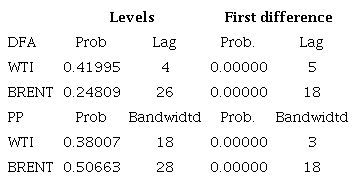
Table 2 shows the descriptive statistics of stationary continuous returns.

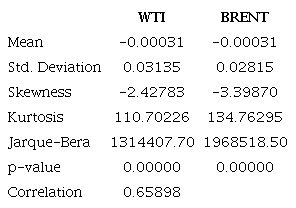
The Jarque-Bera test rejects, in both cases, the null hypothesis that oil returns are distributed as a normal one. This justifies the use of model (3) because, although the disturbances are assumed to be normal, by including the TGARCH model and the break term, the resulting returns are not normal and with wider tails as shown in the kurtosis estimate for both series. Similarly, skewness is positive demonstrating that there is a bias to the right side distribution and that, therefore, there is a probability of having positive extreme returns greater than the probability of having negative extreme returns.

The correlation between the two returns is very high 65%, which establishes strong linear dependence between the two crude references.

The Box-Jenkins methodology is used and the optimal p and q values in the conditional mean are null. This tells us that the estimated conditional mean is a constant with respect to time. The procedure is extended and TGARCH models are estimated for each oil return without considering the jump. The results of the TGARCH (1,1) estimate as in (7) are presented in Table 3. The estimation and p-value for the parameters of the mean equation (upper panel), volatility equation (second panel) are shown.

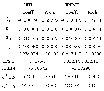
Standardized residuals and squared standardized residuals have a white noise behavior verified by the respective correlograms. Table 3 presents Ljung-Box statistics as well as their order 12 p-value for standardized residuals and squared standardized residuals, thus verifying the goodness of fit of the model for both WTI and BRENT return cases. The variance parameters are statistically positive, and for both cases the leverage effect measured by the $\gamma$ parameter is confirmed.

This parameter is also statistically positive and indicates that when there is a drop in returns, which may be due to market participants getting nervous, volatility increases.

Figure 1 shows the volatility of oil returns obtained from TGARCH models where there are abrupt changes in some parts of the graph.

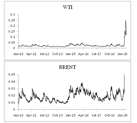
One of the most important changes in crude oil volatility happened in 2014 when prices plummeted for much of the year due to several reasons ranging from geopolitical situations, changes in OPEC targets and overproduction of some countries like the United States, creating an oversupply thus pushing returns downwards.

Another important change in crude oil volatility happened in the first months of 2020, possibly due to the covid-19 pandemic.

These information shocks may be overestimating volatility and can be studied by incorporating the jumps into the TGARCH models estimated above. The results of estimating the parameters of the TGARCH(1,1) model incorporating jumps as in (3) and estimating the conditional probability of jumps for the three different intensity distribution functions are presented in Table 4. The estimation was carried out for the period from January 2010 to December 2019, leaving the period from January to May 2020 to evaluate the performance of the models.

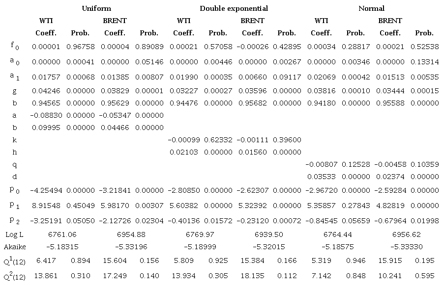
The estimator and p-value are shown for the parameters of the mean equation (upper panel), the volatility equation (second panel), specific parameters of each jump distribution (third panel), and parameters of the conditional probability of jumps (fourth panel).

Again, the goodness of fit of the model is done by verifying that the correlograms of the standardized residuals and the squared standardized residuals behave like white noise. Table 4 presents Ljung-Box statistics as well as their order 12 p-value for standardized residuals and squared standardized residuals, thus verifying the goodness of fit of the model for each of the three returns models for WTI and BRENT.

Static (one period forward) and dynamic predictions (several periods ahead) are made to verify the adjustment with a control sample from January 2010 to December, 2019 and a treatment on which predictions are made from January, 2019 to May 29, 2020. The results of estimating the equation

is reported in Table 5. The joint null hypothesis test statistic that the constant is zero and the slope is one is presented for the simple regression between performed and estimated variance. In parentheses is the p-value.

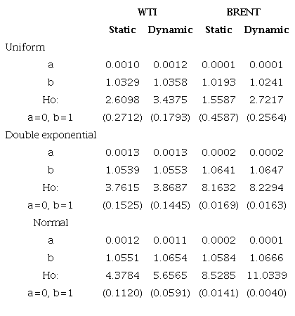
Squared demeaned oil returns are considered for realized data. As predicted data, the conditional variance prediction for each model is taken.

The results show that for both static and dynamic predictions horizon, the Uniform and Double exponential models are in a good fit, since the constant in the regression model cannot be rejected as zero and slope one. For dynamic prediction normal model, the null hypothesis that the constant is zero and the slope one is rejected.

The mean square prediction error (MSPE) and the mean absolute prediction error (MAPE) calculated as follows: are also reported in Table 6.

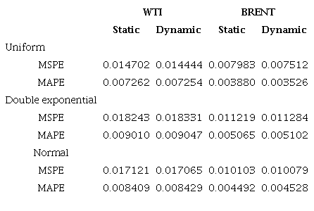
These results show that in the MSPE case, the model with the lowest prediction error for WTI and BRENT is the simplest with a uniform jump distribution, followed by the model with a normal distribution. In the case of HMAE, the results are similar.

According to the logarithm measurements of the likelihood function, the model with double exponential jump distribution function is best for WTI and the normal jump distribution model is best for BRENT followed by uniform distribution.

It is noted that the coefficients of the conditional probability equation are significant in all cases except for the p₁ coefficient (autoregressive part) of the uniform and double exponential models for WTI returns, this tells us that the conditional probability of jumps, in general, has an autoregressive positive behavior, then the probability of jumps has a positive effect on the probability of jumps in the next period, i.e. there are elements of a possible discontinuity in price volatility compared to the previous period and may follow or cause other unexpected rapid changes. The p₂ parameter is negative, therefore the intensity of the jump in the previous period has a negative effect on the probability of jumping this tells us that abnormal information in previous periods has already been incorporated into crude oil prices.

Figure 2 shows the conditional jump probability plots for WTI (left) and BRENT (right) with uniform (top), double exponential (center), and normal (bottom) jump distribution functions.

Figure 2 shows an increase in conditional probability, regardless of crude oil price volatility. This increase in probability, due to abnormal information, began with a drop in price in the last half of 2014. Between June 2014 and January 2015, crude oil prices fell by more than 50%, related to unexpected growth in U.S. oil production, as well as increased production in Russia and Canada. For the following months, conditional probabilities follow average behavior until January 2016 where they fall, this tells us that markets have incorporated that abnormal information and volatility as a measure of dispersion and risk is on track. Causes of these declines in late 2015 and early 2016 are the economic slowdown, at the time, of the Chinese economy, as well as fractures among OPEC members, Iran's oversupply due to the lifting of economic sanctions and again, overproduction in the United States and, the strength of the dollar.

On the other hand, the conditional probability of jumps from 2016 is low and volatility continues its normal course in the market.

Today, the price of oil has a significant effect on the economic development of countries and companies themselves. Understanding the dynamics of its behavior is then fundamental, mainly for many economies and companies that are vulnerable to price hikes and declines. Therefore, developing a better way to describe its stochastic behavior will enable the formulation of better public policies.

Describing the stochastic dynamics of crude oil prices, in addition to its effect as a raw material, will also help in making better decisions by using it as an underlying asset in financial markets through investment instruments such as derivatives.

Some of the typical characteristics of financial asset returns are also valid for oil returns. The distribution of oil price returns has leptokurtosis, i.e. wide tails, which means that there is a greater chance of extreme returns, whether positive or negative. It is also presented the leverage effect that occurs when prices go down and volatility in oil returns increases. One more feature is the volatility clustering in which volatility is grouped, if there is high volatility one day there will be similar volatility the next day. These features are described with TGARCH models. But when prices are exposed to abnormal information, jumps arise, which causes the volatility at that time not to be grouped and a greater variation occur, causing the tails of the returns distributions to be even wider.

In this work, we investigate the role played by volatile oil returns and unexpected rapid changes. Our results, based on daily oil price data, support the inclusion of TGARCH models coupled with jumps. The main contribution of this work relies in adding the conditional probability of jumps which we modeled as an autoregressive behavior. It was found that the probability of conditional jump depends on the probability of jump in the previous period and depending on it in the previous period and the size of the jumps in the previous period. The effect of the probability of jumps in the previous period on the current one is positive indicating that there are elements of a possible discontinuity in price volatility compared to the previous period; abnormal information, if it existed, can follow or cause other unexpected rapid changes. The effect of the size of jumps in the previous period on the current conditional probability is negative showing that the intensity of the jump in the previous period has a negative effect on the probability of jump, this means that abnormal information in the previous periods has already been incorporated into crude oil prices for the following periods.

Finally, we must emphasize that other studies seem necessary to understand oil movements in developing economies. Not only for oil-exporting economies but also for oil importers, these studies may be relevant. In particular, we believe that such studies should focus on the relationship between the price of oil and other macroeconomic variables and estimate the behavior with bivariate distributions and continue with the time series models of the ARCH/GARCH family or models of stochastic volatility, but incorporating the possibility of jumps.